Getting DNA copy numbers without control samples

(1)

S O F T W A R E A R T I C L E

Open Access

Getting DNA copy numbers without control

samples

Maria Ortiz-Estevez

1,2

, Ander Aramburu

1

and Angel Rubio

1*

Abstract

Background: The selection of the reference to scale the data in a copy number analysis has paramount importance to achieve accurate estimates. Usually this reference is generated using control samples included in the study. However, these control samples are not always available and in these cases, an artiﬁcial reference must be created. A proper generation of this signal is crucial in terms of both noise and bias.

We propose NSA (Normality Search Algorithm), a scaling method that works with and without control samples. It is based on the assumption that genomic regions enriched in SNPs with identical copy numbers in both alleles are likely to be normal. These normal regions are predicted for each sample individually and used to calculate the ﬁnal

reference signal. NSA can be applied to any CN data regardless the microarray technology and preprocessing method. It also ﬁnds an optimal weighting of the samples minimizing possible batch eﬀects.

Results: Five human datasets (a subset of HapMap samples, Glioblastoma Multiforme (GBM), Ovarian, Prostate and Lung Cancer experiments) have been analyzed. It is shown that using only tumoral samples, NSA is able to remove the bias in the copy number estimation, to reduce the noise and therefore, to increase the ability to detect copy number aberrations (CNAs). These improvements allow NSA to also detect recurrent aberrations more accurately than other state of the art methods.

Conclusions: NSA provides a robust and accurate reference for scaling probe signals data to CN values without the need of control samples. It minimizes the problems of bias, noise and batch eﬀects in the estimation of CNs. Therefore, NSA scaling approach helps to better detect recurrent CNAs than current methods. The automatic selection of references makes it useful to perform bulk analysis of many GEO or ArrayExpress experiments without the need of developing a parser to ﬁnd the normal samples or possible batches within the data. The method is available in the open-source R package NSA, which is an add-on to the aroma.cn framework. http://www.aroma-project.org/addons.

Keywords: SNPs, Normalization, Scaling, High-throughput data, Batch eﬀects

Background

A DNA copy number aberration (CNA) is a patholog-ical ampliﬁcation or deletion of a part of the genome (a chromosome, one of their arms or a segment) which has been related to cancer development. In CNAs, DNA copy numbers (CNs) may be larger (gains and ampliﬁcations) or smaller (deletions and homozygous deletions) than the normal state (CN=2).

CNAs can be measured using single nucleotide poly-morphism (SNP) arrays. Although the initial application

*Correspondence: [email protected]

1Group of Bioinformatics, CEIT and TECNUN, University of Navarra, San Sebastian, Spain

Full list of author information is available at the end of the article

of these arrays was genotyping, they can also be used to calculate the CN estimates. Besides, regions with LOH (Loss of heterozygosity), which are zones of the genome that show no heterozygous SNPs, can be found using these arrays.

The number of SNPs in the arrays range from the ini-tial ones which interrogate around 10,000 SNPs, to the newest ones which interrogate several millions of SNPs. The GWS arrays from Affymetrix, in addition to SNP probes, include non-polymorphic probes (known as CN probes) for analysis of Copy Number Variations (CNVs). In order to deal with Affymetrix SNP arrays it is required to apply several low level processes, namely, background removal, calibration, normalization and summarization [1]. The final results from these steps are two values (θA

(2)

andθB) for each SNP probeset which are approximately proportional to the number of copies of each allele. On the other hand, the CN probes of the latest arrays have a sin-gle value (θT) proportional to the total number of copies. The proportionality constant is unknown and diﬀerent for each SNP probeset and CN probe.

As previously stated, CNAs occur in segments of the genome. In order to ﬁnd these aberrated regions, it is necessary to compute the scale factor which relates sum-marized SNP signals (θA and θB) and CN values (CNA

andCNB) for each SNP. If there are control samples in the study, the computation of the scale factor is straighfor-ward: two over a robust average of(θA+θB)in the control samples [2-6] .

In this work it is assumed that a control sample has neu-tral copy number with no LOH in its whole genome. Of course, there can be CNVs in a control sample but, for sake of clarity, they are not considered here.

Unfortunately, there are many experiments that do not include control samples due to the difficulties to find them or simply to reduce experimental costs. In these cases, researchers opt for either using control samples from a public dataset or calculating a robust reference using the tumoral samples available in the experiment (implicitly assuming that for each SNP most of the tumoral sam-ples have neutral CNs). However, as it will be shown, using samples from different labs can increase the noise in the CN estimations and assuming that SNPs have neutral CNs in most of the samples, although usually works, can introduce bias in the copy number estimations hiding real CNAs or even creating false ones, mostly when there is a recurrent aberration.

We propose an algorithm termed NSA (Normality Search Algorithm) that generates for each sample the cor-responding reference without the need of control samples. Within each of the samples (control or tumoral) NSA

(3)

Table 1 Level of Heterozygisity

Genotype CN LH

- 0 NAN

A,B 1 0

AB 2 1

AA,BB 2 0

AAB,ABB 3 2/3

AAA,BBB 3 0

AAAB,ABBB 4 1/2

AAAA,BBBB 4 0

AABB 4 1∗

LHof each genotype-CN pair for CNs in a pure tumor sample.

*_{The last genotype marked with an asterisk, implies a simultaneous alteration in}

both chromosomes which is very unlikely to occur.

detects regions with neutral CNs (CN=2) and no LOH.

Using these normal regions, the reference is calculated and used to scale the data through both SNPs and samples. We will show that NSA is able to correctly scale the CN estimates even if there are no control samples in the exper-iment. In addition, NSA is able to infer the batches within an experiment and ﬁnd a proper weighting (diﬀerent for each sample) to calculate the references.

The core of the NSA algorithm is the detection of nor-mal regions in the genome. The developed method is based on the comparison of the signals for both alleles in each SNP. Heterozygous neutral copy number SNPs (HNCNs) have similar signals for both alleles (θ_jA_,_i θ_jB_,_i) and their total copy number is two. For the majority of aberrations (amplifications, deletions or LOH), one of the alleles will have a larger signal than the other since the number of copies is different for each of them. AABB (or AAABBB) genotypes are very unlikely (except in mul-tiploid cells) since it implies an amplification of both chromosomes and this occurs much less often than aber-rations that involve only one of the chromosomes [7]. The nuclear assumption of NSA is that a SNP that have simi-lar signals in both alleles (θ_jA_,_i θ_jB_,_i) is probably a HNCN. NSA assumes that regions enriched in SNPs with similar signal for both alleles have neutral total CNs and no LOH. Once NSA has inferred the normal regions, it also computes the optimal weights to calculate the reference using a weighted median. These weights are different for each sample and strongly related with the batches (set of samples that share some characteristics such as day of hybridization, lab, person, etc) in which the samples were hybridized. Finally, the reference is calculated and the data scaled across both SNPs and samples.

NSA has been implemented in the aroma.cn framework and memory requirements are modest even for a large number of samples. Moreover, it is independent of both the preprocessing method or the microarray technology.

Implementation

NSA is a population-based multi-array method for scal-ing any SNP & CN array technology, e.g. Affymetrix and Illumina. It identifies the normal regions within the samples, finds optimal weights to account for hybridization batches, calculates the corresponding references and, finally, performs a two-dimensional scaling.

Data

We applied NSA to five different datasets. The first one is a subset of a Gliobastoma Multiforme (GBM) experi-ment that includes 64 tumoral samples [8] hybridized to Affymetrix Mapping 50K Xba array. The second one is a Prostate Cancer analysis with 20 tumoral and 20 control samples [9] hybridized to Affymetrix Mapping 250K Nsp array, the third one is a subset of 50 Lung Cancer and 20 control samples from [10] hybridized to Affymetrix GWS 6.0 array. The fourth one is a subset of an Ovar-ian Cancer experiment that includes 72 tumoral samples and 57 control samples [11] and, finally, the fifth one is a subset of HapMap samples [12]. It is shown here that, for these datasets, NSA provides more accurate and precise CN estimates than other state of the art scaling methods.

The input data of NSA are the summarized probe sig-nals (θA and θB) calculated using any summarization method such as dChip [13], RMA [14], CRMA v2 [1],

(4)

ACNE [15], CalMaTe [16] for Affymetrix arrays or the one developed by [17] for Illumina technology. From these allele specific probe signals the fractions of the B-allele (β =θB/(θA+θB)) are obtained. CRMA v2 pre-processing methods have been applied to all the datasets. In the summarization step, ACNE (for Affymetrix Map-ping 50 and 250K arrays) and CalMaTe (for the GWS6.0 arrays) were chosen because provide more accurate allele specific CNs.

Detection of neutral DNA copy number regions

The main assumption of NSA is that gains of both chro-mosomes in a tumor sample are very unlikely to occur.

It is shown in [7] that (for GBM) only 3% of the aber-rations occur in both chromosomes. Therefore, we con-sider that if both θA and θB are approximately equal, the SNP is likely to be heterozygous with CN equal to 2 (i.e. it is a HNCN). Since CNAs occur in segments of the genome, the homozygous SNPs within a region enriched in HNCNs will probably also have neutral CNs. In order to quantify how similar the signals of both alle-les are, we use the termlevel of heterozygosity(LH) which stands for a continuous approximation to the heterozy-gosity of a SNP (notice that this level of heterozygosity

does not have anything to do with the same term in population genetics).

(5)

Level of Heterozygosity

By deﬁnition theLHfor a given SNPj(j=1. . . J) in a sample

i(i=1. . . I) is calculated as

LHj,i=2min(θjA,i,θjB,i)/(θjA,i+θjB,i) (1)

whereθ_jA_,_iandθ_jB_,_iare the corresponding signals of A and B alleles for SNPjin sampleiand they are expected to be proportional to their CN values (CN_jA_,_iandCN_jB_,_i). IfLHj,i is close to 1 (θ_jA_,_i θ_jB_,_i), SNPjis expected to be heterozy-gous in samplei. On the other hand, if it is close to 0 it means that one of the signalsθ_jA_,_iorθ_jB_,_iis close to zero and, therefore, either the SNPjis homozygous in samplei, or that there are more copies of one allele than of the other (which occurs in an ampliﬁed zone). The values of theLH

matrix (dimensions JxI) are within 0 and 1. Alternatively,

LHcan be deﬁned as

LHj,i=2min(βj,i, 1−βj,i) (2)

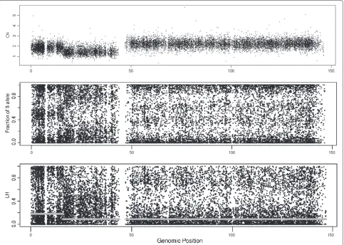
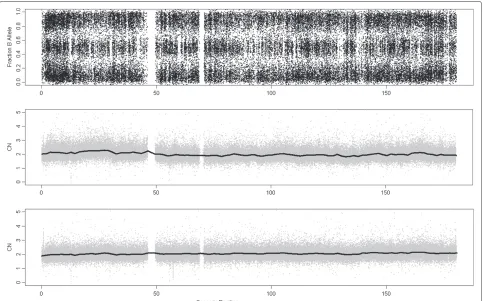
whereβj,i=θjB,i/(θjA,i+θjB,i)are the fractions of the B-allele. Figure 1 displays the CNs, the fraction of B-allele (β) and

theLHof chromosome 8 in sample GSM318736, from the

Prostate Cancer experiment. The top panel shows three diﬀerent zones in this sample: a normal zone in the begin-ning of the chromosome (CN=2, from 0 to 20 Mb), a deletion in the zone of theparm closer to the centromere (CN=1, from 20 to 45 Mb) and a gain in theqarm of the chromosome (CN=3, from 45 to 147Mb). These regions

can be inferred from the CN plot, but also from theβ

plot (middle panel). On the other hand, in the bottom panel, theLHplot shows two clouds in the normal region: one is centered at 0 and the other at 1. The distribution is also bimodal for 3 copies, but the peaks for the dis-tributions are, in this case, about 0 and 0.7. The density function ofLHin a deletion presents a plateau for low val-ues (close to 0), and it is unimodal if there is no normal contamination.

HNCNs have a distribution that peaks at LH = 1

(the place whereθ_A = θ_B). The density function ofLH

for homozygous SNPs has a peak close to 0 (row two in Table 1). The speciﬁc position of the peak depends on the summarization method, especially on how well the method deals with cross-hybridization between probes that measure diﬀerent alleles. The expected values ofLH

for the SNPs with CN diﬀerent to 2 are shown in Table 1 (The last genotype marked with an asterisk, implies a simultaneous alteration in both chromosomes which is very unlikely to occur).

Selecting Heterozygous SNPs with Neutral CNs (HNCNs)

Using Table 1, a thresholdLHthhas been selected to dis-cern whether the corresponding SNP is HNCN or not. The most critical case to discern from a normal region (using theLHvalue) is a zone with 3 copies. The expected

LHvalue is around 2/3 for a perfect summarization model with a pure tumor sample. If there is contamination from the surrounding normal tissue, this value will be larger. Because of this, a suitable threshold is 5/6 (the middle

(6)

Figure 5DNA copy numbers using MHS (291 samples where 59 are control samples from HapMap, used to calculate the reference) and NSA (reference using “normal” zones within tumoral samples (232 samples)) for chromosome 5 in sample GSM638958 from the Lung Cancer dataset hybridized to GenomeWideSNP 6.0.

point between the expected value for normal heterozy-gous calls and the value for 3 copies).

Figure 6ROC comparison with scaled data (Lung Cancer dataset, sample GSM638958, hybridized to GenomeWideSNP 6.0 array).We have used the region where there is a change from 2 to 3 copies, around position 30Mb, that appears in Figure 5. For the analysis, we have included the SNPs that surrounds the copy number change (specifically from 0 to 45 Mb). The SNPs within a safety zone from 25Mb to 35 Mb are not considered in the analysis because it is difficult to discern the exact position of the change. The SNPs located upstream the change point are considered to have total CNs smaller than the SNPs downstream the change point. For this particular sample (in the studied jump), NSA differentiates the two regions better than MHS.

Once the threshold is set, the SNPs withLHvalue over it are labeled as HNCN (LH=1) and the others as non-HNCNs (LH=0). A segmentation algorithm is applied to these binary data to ﬁnd zones enriched in HNCNs. We used a variant of CBS in which the input are binary data [18,19], although other methods could be applied (using for example Hidden Markov Models [20]).

In the aforementioned Figure 1, the thick gray lines in the bottom panel represent the different segments pre-dicted by CBS. The yaxis represents the proportion of HNCNs SNPs in the segment. It can be observed that CBS detects 2 different segments, corresponding to the two states (normal and aberrated). In other samples, segmen-tation also differentiates between aberrations (deletions and gains) assigning them a different value since the pro-portion of SNPs whoseLHis above the threshold can be different, but this fact does not affect the method.

Labeling normal segments

On average, 27% of the SNPs in a HapMap sample are het-erozygous. Therefore, ideally, the proportion of HNCNs in a normal region would be around 27%. On the other hand, the proportion of HNCNs should be ideally close to 0% in an aberrated region. We have selected a thresh-old in the middle point (13.5%). The larger the threshthresh-old, the more likely the selected segments have neutral CNs. However, some normal regions can be missed because of noise or simply because the regions include many SNPs with onerare variant.

For example, consider the initial part of the p arm

(7)

amplified. The density function for the normal zone has more SNPs with LH closer to 1 than the amplified region. In this particular case, 18.3% of the SNPs are above the threshold set in the previous section. For the 3 copies region, only 8.6% of the SNPs have LH above the thresh-old. The difference between both regions is large enough, so that, the algorithm is not sensitive to a particular selection of the threshold.

If the array of the experiment includes SNP and CN probes (GWS 5.0 or GWS 6.0), then the corresponding status (neutral copy number or not) of the CN probes is inferred from the status of the segment where they are located (that has been computed using the SNP probes).

Copy number data scaling

The ﬁnal processing of NSA includes two scaling steps, one by SNPs and another by samples.

Scaling by SNP

NSA implements two methods (user-selectable) to com-pute the references: the first one uses standard medians and the second one uses weighted medians to minimize batch effects. In this second method each sample has a different computed reference.

For the ﬁrst method, the reference is computed by using the median of the signals of the samples labeled as normal for each SNP. In the second case, a diﬀerent algorithm (described in the following section) estimates some weights that are used to compute the reference for each SNP and sample using weighted medians [21]. It also

uses only the samples labeled as normal for each SNP to compute the reference.

Scaling by sample

The algorithm computes for each sample the median of the CNs of the SNPs assumed to be normal and re-scales all the data so that the median of the normal zones for each sample is 2.

The two scaling steps of the proposed normalization is similar to a median polish in which only the SNPs which are labeled as normals are included in the computation.

Algorithm

The procedure that involves both scaling steps is the following:

1. Get the reference signal for every SNP computing:

Ref_jSNP=mediani∈I(SLHj,i)(θ

(1)

j,i ) (3)

whereθ_j(_,1_i)=θ_jA_,_i+θ_jB_,_iis the sum of the signals of both alleles andI(SLHj,i) is an indicial matrix of the

samples (for SNPj ) that have been labeled as normal in that position.Ref_jSNPis the computed reference for SNPj, taking the medians by SNPs. If the batch eﬀect removal (BER) method is used, this step converts into

Ref_jSNP_,_i =wmedian_k∈I(SLHj,k)(θ

(1)

j,k ,γi,k). (4)

wherewmedian stands for the weighted median using weightsγ_i_,_k. Notice that the reference is diﬀerent for each SNPj but also for the same SNP in

(8)

Figure 8ROC comparison with scaled data (Lung Cancer dataset, sample GSM639066, hybridized to GenomeWideSNP 6.0 array).We have used the region where there is a change from 3 to 2 copies, around position 65Mb, that appears in Figure 7. For the analysis, we have included the SNPs that surrounds the copy number change (speciﬁcally from 0 to 100 Mb). The SNPs within a safety zone from 60 Mb to 75 Mb are not considered in the analysis since includes a deleted region. The SNPs located upstream the change point are considered to have total CNs larger than the SNPs downstream the change point. For this particular sample (in the studied jump), NSA diﬀerentiates better than MHS between the two regions.

a diﬀerent samplei, since the weights of the median (γ_i_,_k) are diﬀerent for each sample. These weights are computed by the algorithm described in the

following section.

2. Normalization of the signals across SNPs. For each SNP in every sample

θ_j(_,2_i)= 2θ

(1)

j,i

Ref_jSNP₍_,_i₎ (5)

The values ofθ_j(_,2_i)will be close to the real CNs. The reference will be diﬀerent for each sample if the batch eﬀect removal method is used.

3. Get the reference signals for every sample:

Ref_isample=median_j∈I(SLHj,i)(θ

(2)

j,i ) (6)

Ref_isampleis the average value (using medians) of the normal segments of the genome. This value is expected to be close to 2. In order to ensure this, the following (and last) step scales the samples

accordingly.

4. Normalization of the signals across the samples. For each sample, in every SNP

θ_j(_,3_i)= 2θ

(2)

j,i

Ref_isample

(7)

The values ofθ_j(_,3_i)are the ﬁnal estimates of NSA for the total CN values.

These steps should be repeated until convergence but improvement is negligible after the ﬁrst iteration (average copy number changed about 0.001 copies in the exam-ples).

Computation of weights for batch eﬀect removal

Batch eﬀects have proved to have paramount importance in the analysis of SNP arrays [22,23]. The particular char-acteristics of NSA algorithm helps to develop an algorithm to minimize them. The overall idea is that, since NSA identiﬁes normal zones that are expected to have neu-tral CNs, the reference can be selected so that, for these normal zones, the estimated copy number is close to 2.

The procedure is the following. First of all, a set “S” of SNPs is selected. This set must include a suﬃcient number of normal SNPs to capture the relationships between the arrays. These SNPs are selected from normal regions in

(9)

most of the samples. Although for some studies there are no normal SNPs for all the samples, the SNPs in “S” are selected so that they appear as normal in as many samples as possible.

For SNPs in “S” that are not located in normal regions in any of the samples, their values are substituted by the references using standard medians, the signal used by the algorithmθˆis

ˆ θ_j∈S,i=

θ_j∈S(1)_,_i, ifi,j∈I(SLHj,i)

Ref_j∈SSNP, otherwise (8)

Using these values, the weightsγ_i_,_k to compute the

ref-erence for each sample i are estimated by solving the

following optimization problem

min

γi,k ||

log(θˆ_j∈S_,_i)− I

k=1,k=i

γ_i_,_klog(θˆ_j∈S_,_k)|| (9)

subject to

γi,k>0,γi,i=0 (10)

implicitly assuming that the reference for log(θ )ˆ is

γ_i_,_klog(θˆ_j∈S_,_k), i.e. a linear combination of the logarithm of the signals for each sample. The restrictions impose that 1) sampleiis not used to compute its own reference and 2) only positive weights are allowed, i.e. if samplesiandkare so diﬀerent that the corresponding coeﬃcientγ_i_,_kis nega-tive, samplekis not used to build the reference of sample

iinstead of giving it a counter-intuitive negative weight.

Figure 10DNA copy numbers using ACNE, ACNE+NSA and CN5 and B Allele Fraction for chromosome X in sample

(10)

Figure 11ROC comparison with scaled data (GIGAS HapMap dataset, sample

GIGAS g GAINmixHapMapAffy2 GenomeWideEx 6 A04 31266, hybridized to GenomeWideSNP 6.0 array).We have used the initial region of chromosome X, where there is a change from 2 to 1 copy, that appears in Figure 10. For the analysis, we have included the SNPs that surrounds the copy number change (specifically the first 1000 SNPs, ordered by genomic position). There is no safety zone in the analysis. The SNPs located upstream the change point are considered to have total CNs larger than the SNPs downstream the change point. Again, for this particular sample (in the studied jump), NSA differentiates better than ACNE (in this case, “MTS”) and CN5 (in this case, “MCS”).

This optimization is a quadratic programming (QP) problem. Instead of using a standard QP algorithm (quite time consuming) we have iteratively solved the minimum squares problem. In each step, the algorithm removes the samples whose weights are negative in the solution.

Any linear combination such as γ_i_,_klog(θˆ_j∈S_,_k), can be interpreted as a weighted mean multiplied by an addi-tional factor (the sum of the weights). In this particular case, since the data are further normalized by samples, this additional factor is computed and taken into account in the “scale by samples” step. In addition, instead of using the weighted mean, we used a weighted median to increase the robustness and withstand the presence of outliers. Since the median and the logarithm are inter-changeable operators, the suggested reference is

Ref_jSNP_,_i =wmedian_k∈I(SLHj,k)(θ

(1)

j,k ,γi,k). (11)

Using this formula, each of the computed γ_i_,_k is the weight of the normal regions of samplekto compute

ref-erence for sample i using a weighted median. For each

SNP j, only the samples that are expected to be

nor-mal are included in calculation of the median using the corresponding weights.

Results

In this part, it is shown that the results using NSA out-perform the use of control samples from a different lab or using a robust median of the tumoral samples (which are the most used methods). This improvement in perfor-mance appears both in noise and bias. Since there is not a ground truth to compare against, we have used three indi-rect aspects to state the performance: the ability to find CNAs along the genome, the quality of the estimated CNs in regions that are known to be normal and the ability to find recurrently aberrated regions.

Eckel-Passow et al. [24] shows a comparison among

different summarization algorithms. It describes four summarization methods [2-5]. Within these methods, there are only two different algorithms for scaling: using the median (of some of the samples) and a linear model. The summarization methods used here (ACNE and CalMaTe), internally implement a calli-bration that is in fact a linear model. In addition to the methods described in [24], dChip [6] imple-ments a trimmed mean of the samples if no ref-erences are provided, LaFramboise [25] fits a non-linear model using the information from control sam-ples, Nannya et al [26] propose to use the m con-trol samples most similar to the sample under study. In the end, the suggested methods to scale the sam-ples (except [26]) are simply the computation of a robust average (i.e. the median or a trimmed mean) of some of the samples. As will be shown later, our approach to remove batch effects resembles Nannya’s but focusing only on the normal zones within the tumor samples.

We have compared four diﬀerent possibilities to select the samples to build the references. These scaling meth-ods depend on whether control samples are available or not and on the laboratory where the control samples (if any) were hybridized. The ﬁrst algorithm under study can be applied to a dataset which includes control samples from the same lab. In this case, for each SNP, the median of the values of the control samples is used as reference i.e, the median of (θ_CA_,_i+θ_CB_,_i) whereCis a subset of control samples within the experiment. We named this algorithm MCS (median of control samples). This is the method of choice suggested by all the referred methods if control samples are available.

(11)

some vignettes of the package aroma.aﬀymetrix [2]. And, ﬁnally NSA, which calculates the reference based on the predicted normal regions within the tumoral samples.

Ability to ﬁnd recurrent aberrant regions

We have focused this section on the detection of recurrent alterations since it is the aim of many CN analysis.

The analyzed experiment is the GBM dataset (64

tumoral samples [8] hybridized to Aﬀymetrix

Map-ping50K 240Xba). The data were analyzed using

CRMAv2 pre-processing and ACNE summarization method. Once theθ values were obtained, the data were scaled using both MTS and NSA. In addition, we per-formed the same analysis taking HapMap samples as references (MHS).

After applying the three scaling methods, the CN esti-mates were segmented using CBS [18] and then, the recurrent aberrant regions were calculated using GISTIC [27].

GBM has been deeply studied by diﬀerent groups [8,28], and it is known to present strongly recurrent aber-rations. For example, in GBM there is a well known

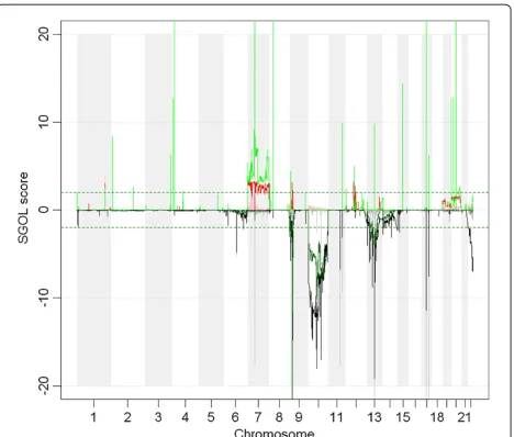
recurrent ampliﬁcation in 7q and a deletion of almost the whole chromosome 10 [28]. Figure 2 shows the recurrent aberrations found using the median of the tumoral samples (MTS), shown in thick red and grey, the ones obtained from NSA (lines red and black) and MHS (green and dark green). Using MTS, the

aber-rated region 7q does not only appear to be ampliﬁed

but also deleted. This recurrent deletion is an artiﬁ-cial aberration originated by the bias of the estima-tion of the reference. Since the recurrent ampliﬁcaestima-tion

in 7q occurs in more than half of the samples, the

MTS estimates of the reference for these loci are larger than the real ones. In turn, the scaling process pro-vides smaller copy number values than expected for these loci. This is a general trend: in recurrent amplifications, MTS estimates are larger for neutral copy number loci than expected. This bias makes the amplification less prominent and the statistics less significant. The oppo-site effect can also be seen in chromosome 10, which is known to be recurrently deleted. Using MTS, both a recurrent amplification and a recurrent deletion appear in chromosome 10.

(12)

On the other hand, in both chromosomes 7q and 10, NSA and MHS provide more significant values for the aberrations (the amplified and deleted regions have higher q-values) and no artificial aberrations appear. The per-formance in terms of identifying recurrent aberrations is similar for both algorithms. Nevertheless, we have to fine-tune the low-level analysis using MHS since a very strong bias appears in the CN estimates (that NSA does not present because of the second stage of the algorithm -scale by samples).

Ability to ﬁnd CNAs along the genome

We have performed this comparison in two cancer datasets, Prostate Cancer and Lung Cancer. In addition, we have analyzed the chromosome X in some HapMap samples to check if NSA is able to uncover which samples

have two copies (female samples) and, using the ﬁrst auto-somic region of this chromosome, compare the ability to ﬁnd a copy number change.

Prostate cancer analysis

The Prostate Cancer dataset is hybridized to Aﬀymetrix Mapping250K Nsp [9]. We compared the NSA results with MTS, MCS and MHS. It is reminded that MCS needs more hybridizations than the other methods. This analy-sis is focused on ﬁnding aberrant regions in order to show which method detects CNAs more accurately.

Figure 3 presents the DNA CNs of chromosome 8 for sample GSM318766 obtained using the different scaling methods. It is not possible to pinpoint clear differences from these figures, except for the MHS method which is clearly noisier than the others in this example.

(13)

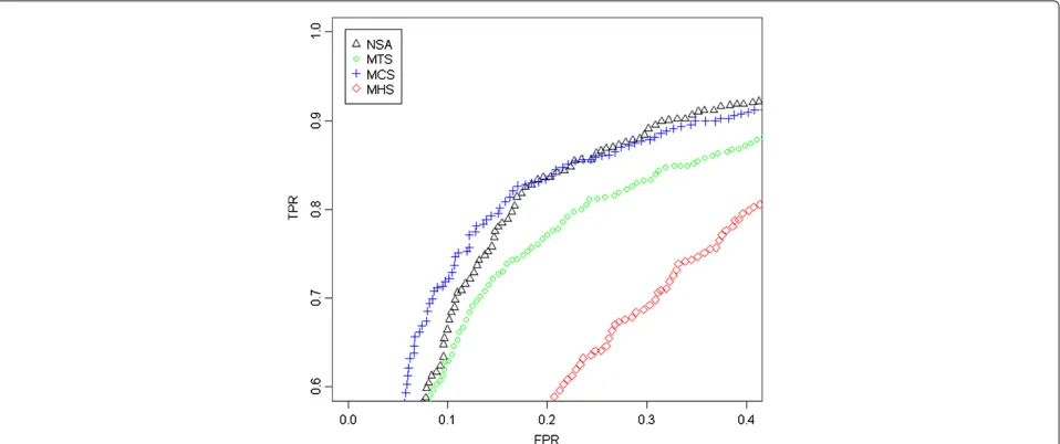
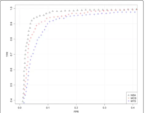
In order to quantify the ability to find CNAs we have generated a ROC curve (Figure 4) for the region that changes from 1 to 2 copies, around position 32Mb (Figure 3). The SNPs located downstream the change point are considered to have a larger total CN (which have neutral CNs) than the SNPs upstream the change point (deleted region). For any threshold in the CNs there are true positives TP (SNPs in the normal region that are above the threshold), false positives FP (SNPs in the deleted region that are above the threshold), true nega-tives TN (SNPs in the deleted region below the threshold) and false negatives FN (SNPs in the normal region that are below the threshold). The FPR = FP /(FP + TN) and TPR = TP /(TP + FN) can be evaluated at different thresholds. The ROC curve is the plot of TPR against FPR for differ-ent thresholds. A perfect classification method provides large TPRs for low FPRs. The worst classification method (random selection) is a straight line from (0,0) to (1,1). This evaluation method was also used by Bengtsson et al. in [1] and it is deeply explained in their corresponding Supplementary Notes.

For this analysis, we have included the SNPs that sur-round the CN change (speciﬁcally from 20 to 45Mb). Since the exact position of the change is diﬃcult to locate,

Figure 14ROC comparison with scaled data (Ovarian dataset, sample GSM492511 IC318T, hybridized to GenomeWideSNP 6.0 array).We have used the region where there is a change from 3 to 2 copies, in the begining of chromosome 1, that appears in Figure 13. For the analysis, we have included the SNPs that surrounds the copy number change (speciﬁcally from 60 to 85 Mb). The SNPs within a safety zone from 70 Mb to 75 Mb are not considered in the analysis. The SNPs located upstream the change point are considered to have total CNs larger than the SNPs downstream the change point. For this particular sample (in the studied jump), NSA (with BER) diﬀerentiates better than NSA (without BER) and CalMaTe using control samples as references (MCS).

the SNPs within a safety zone from 30Mb to 34Mb are not considered. This ﬁgure includes some gray zones that illustrate which is the region under study. It can be seen in Figure 4 that MCS and NSA are the ones that best identify this CN change (better TPR for the same FPR). MTS gives intermediate results and MHS performs worse than the rest. We have selected this locus since it is the most promi-nent recurrent aberration for this dataset and has been previously shown to be a frequent aberration in Prostate Cancer [29,30].

Lung cancer analysis

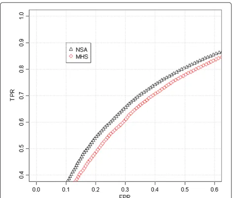
We have also validated NSA with the dataset from a Lung Cancer study [10], hybridized to Aﬀymetrix GenomeWideSnp 6.0. It should be noted that in this study there are 291 samples where 59 are control samples from a diﬀerent lab (one of the authors informed us in a personal communication that they are from HapMap).

Figure 5 shows the CNs of chromosome 5 in sample GSM638958 using MHS (over the 291 samples) and NSA (using the 232 tumoral samples). It can be seen from this ﬁgure that the noise using MHS is again larger than using NSA. The region used here to calculate the ROC ranges from 0 to 45 Mb and the safety region is from 25 to 35 Mb where there is a jump from 2 to 3 copies[31,32]. The ROC curve from Figure 6 shows that NSA performs bet-ter than MHS. Figures 7 and 8 shows a similar behavior in a diﬀerent sample and location.

Chromosome X analysis

(14)

Using this information, we have compared ACNE, ACNE+NSA with CN5 (see Figure 10). CN5 uses the information of sexual chromosomes (i.e. which samples are male and female) to perform the scaling. In this particular analysis, ACNE and NSA do not have this information. Plain ACNE can be considered to scale by using the MTS method (all the samples are used as ref-erence regardless of the sex) and CN5 by using MCS (uses the expected number of copies for female sam-ples). We have analyzed the CN jump located at the end of the PAR1 region of chromosome X in a male sample. This pseudoautosomal region goes from 0.6 Mb to 2.699 Mb. The ROC curve in Figure 11 shows that, ACNE performs worse than CN5 in this particular anal-ysis. However, after correcting ACNE with NSA, its ROC outperforms CN5’s.

CN estimates for normal regions

In the previous paragraphs we have shown that using samples from different labs increases the noise of the estimates. However, it will be shown here that this fact does not only increase the noise but also the bias. We have used again the Lung Cancer dataset hybridized to Affymetrix GenomeWideSNP 6.0 array and chosen a chromosome in a tumoral sample which seems to be nor-mal (since the fracB plot shows three clouds through the whole chromosome, Figure 12). These three clouds corre-spond to SNPs with AA, BB and AB genotypes. Figure 12 shows the CN estimates using MHS (middle panel) and NSA (bottom panel). A wavy effect on the whole chro-mosome appears when using MHS, which does not occur using NSA. This bias that changes along the genome is originated by a wrong computation of the reference.

(15)

Moreover, there is also another bias, which exists even using control samples from the same lab. This bias is generated in the pre-processing step where the samples are normalized. This step performs a transformation on probe level data to make them comparable across differ-ent samples. This transformation can be a quantile scaling or simply a multiplication of the data by a constant. Nev-ertheless, if a large part of the genome in a sample is deleted (amplified), the normalization procedure tends to compensate for this effect and the normal regions of the genome (that ideally have CN=2) are shifted to a larger (smaller) value to compensate for the aberration. This fact induces a bias in the CN estimation. Therefore, if there is a sample with many deletions (or amplifications), the nor-mal regions of these samples have a slightly higher (lower) value than 2.

Behavior in the Presence of Batch Eﬀects

We have also analyzed the ability to remove batch eﬀects using NSA. For this we have used the Ovarian Can-cer dataset [11]. This dataset includes 129 samples (72 tumoral and 57 references, some of them matched) that were hybridized in 13 batches. The number of samples for each of the batches is very diﬀerent to each other rang-ing from 2 samples in one batch to more than 20 samples in another batch. In the case of small batches, the advan-tage of computing the references by batches or taking the experiment as a whole is unclear.

We have applied NSA with batch eﬀect removal on this dataset. NSA’s procedure to estimate the weights is com-pletely blind, i.e., it does not require any information from the user on which are the samples within each batch.

Figure 13 shows the chromosome 1 in sample GSM492511 ICT318T using CRMAv2 plus CalMaTe summarization method and NSA to scale the result. First panel shows CalMaTe using the control samples as ref-erences (taking all of them as a whole) and second and third panel show the scaling after running NSA without and with Batch Effect Removal (BER). It can be seen that the overall noise is slightly smaller using NSA with BER. To quantify this effect, we have also included the ROC curve (Figure 14) of the CN change around position 70 Mb. This ROC confirms what is seen by bare eye: the noise is smaller and therefore, the ability to detect copy number changes improves. We have included also the analysis in a different sample (GSM492507 IC288T) of a change from 1 to 2 copies (Figure 15). This general trend is similar. This copy number change is easier to pinpoint as shown by the upper location of the ROC curve (Figure 16). The behav-ior of NSA (without BER) and MCS is similar. Therefore, NSA can be used safely without the need to provide the control samples to the scaling method.

Figure 17 shows a hierarchical clustering of the correla-tion of the matrix of weightsγ_i_,_k. It can be seen that the

weights are similar for samples hybridized within the same batch. Each batch have a diﬀerent color (gray scale). The shades of gray are ordered by hybridization day.

Discussion and conclusions

This paper describes NSA, an algorithm to scale the sum-marized SNP signals to CN values by finding normal regions within tumoral samples. NSA is platform (Illu-mina or Affymetrix) and pre-processing method (dChip, CRMAv2, ACNE, CalMaTe. . . ) independent. The syn-thetic reference generated by NSA using only tumoral samples gives more accurate results than either using con-trol samples from different labs or using all the tumoral samples. Indeed, NSA results are close to the ones obtained using control samples from the same lab within the dataset. In addition, NSA includes an algorithm to deal with batch effects. It automatically computes an opti-mal reference for each sample (that in our tests is strongly related to the hybridization batches). Batch information is not required to run NSA; the algorithm automatically identifies the proper samples to compute the reference using only the signals of the microarrays. NSA minimizes the problem of bias for samples with a large number of similar aberrations (i.e. most of them are gains or dele-tions). For these samples, the predicted CNs for normal regions tends to compensate the aberration including a

(16)

Figure 17Hierarchical clustering performed on the correlation of the weighting matrix (γi,k) calculated for the Ovarian dataset.This

dataset have been run in 13 batches. Each batch has a diﬀerent color (gray scale). The assigned gray scale is done according to date of hybridization. A gray scale band is added in top of the ﬁgure. It can be observed that the weights are similar for samples hybridized in similar batches.

bias. This is a potential problem that also occurs using MCS (control samples from the same lab). NSA is able to eﬀectively discover the normal regions and uses them to scale the data diminishing any bias that appears in the normalization step.

We have compared NSA with other scaling methods. On one hand, it is important to pinpoint that the number of hybridized samples needed for NSA, MTS and MHS is much smaller than using MCS, since these methods do not need to hybridize control samples from the same lab to create the reference. MHS method seems to be nois-ier which can be an effect of the difference between the protocols or conditions of the labs where the arrays were hybridized. MTS provides biased estimates especially in the case of recurrent aberrations. On the contrary, NSA estimates are similar to the ones from MCS. In addition, NSA provides a way to deal with the unavoidable batch effects of large experiments.

NSA also presents some limitations that are summa-rized here. Ultimately, the identiﬁcation of normal regions relies on the fact that gains in both chromosomes are very unlikely to occur. If this is not the case and a few samples do present ampliﬁcations on both chromosomes,

NSA is still reliable since a robust estimator of the refer-ence (such as the median) can withstand the presrefer-ence of a small percentage of outliers.

The prediction of normal regions can be aﬀected by samples with low tumor purity that can be wrongly included within the normal ones. Again, since the median withstand the presence of errors, it will only aﬀect if most of the samples have very low tumor purity which usually is not the case.

The number of samples used by NSA to build the ref-erence is diﬀerent for each locus. Therefore, the variance of the reference varies on each position. In particular, recurrently aberrated regions have a reference with larger variance than regions that show seldom aberrations.

Since NSA is based on ﬁnding regions enriched in HNCNs, if an aberration occurs in a region with no SNPs (it includes only CN probes), NSA cannot provide an accurate reference for this region.

Similarly, NSA estimates of chromosomesXandY are

(17)

Finally, one potential situation in which NSA could fail is ifallthe samples present an aberration in the same locus. This is very unlikely event but it could potentially occur. Even in this putative case, a few samples hybridized in the same lab can be included in the study to avoid these “emergency cases”.

In spite of these limitations (most of them also present in other scaling methods), NSA is able to ﬁx the problem of ﬁnding recurrent regions and copy number changes when no control samples are available.

If NSA is applied to a dataset with both tumoral and control samples, the detection of CN changes could be even more accurate than using MCS (especially if NSA removes the batch eﬀects) because of having more and (what is more important) more appropriate samples to calculate the references. This fact makes NSA especially convenient to apply to many experiments (in GEO or ArrayExpress) without the need to explicitly state which are the control samples or the batches in the datasets.

In conclusion, NSA can be used to accurately scale sum-marized SNP signals to CNs. It presents less bias and noise than MTS or MHS and needs no control sample hybridization.

Availability and requirements

The proposed NSA method is available in the NSA package implemented in R (R Development Core Team, 2010). This package includes an add on to the high-level aroma.aﬀymetrix framework [33], which allows NSA to be applied to very large SNP data sets. It is publicly available at CRAN repository in a package called “NSA”.

Abbreviations

LH, Level of Heterozygosity; HNCNs, Heterozygous Neutral Copy Number SNPs; CNA, Copy Number Aberration; CNs, DNA Copy Numbers; SNP, Single Nucleotide Polymorphism; LOH, Loss of Heterozygosity; CNVs, Copy Number Variations; NSA, Normality Search Algorithm; BER, Batch Eﬀect Removal; QP, Quadratic Programming; MCS, Median of Control samples; MHS, Median of HapMap samples; MTS, Median of tumoral samples.

Competing interests

T he authors declare that they have no competing interests.

Author’s contributions

MO conceived the idea and jointly with AA developed the add-on to the aroma.cn framework. AR developed the algorithm to account for batch eﬀects. MO, AA and AR wrote the manuscript and developed the software to compare NSA against other algorithms. All authors read and approved the ﬁnal manuscript.

Acknowledgements

The authors would like to thank Luis Montuenga and Maribel Zudaire (“Centro para la Investigacion Medica Aplicada”, CIMA, University of Navarra) for their support and advice in the analysis of the biological consequences of the copy number alterations.

Author details

1_{Group of Bioinformatics, CEIT and TECNUN, University of Navarra, San}

Sebastian, Spain.2_{Computational Biology Group, Celgene Institute for} Translational Research Europe (CITRE), Sevilla, Spain.

Received: 2 December 2011 Accepted: 15 June 2012 Published: 16 August 2012

References

1. Bengtsson H, Wirapati P, Speed T:A single-array preprocessing method for estimating full-resolution raw copy numbers from all Aﬀymetrix genotyping arrays including GenomeWideSNP 5 & 6. Bioinformatics2009,25(17):2149–2156.

2. Bengtsson H, Simpson K, Bullard J, Hansen K:aroma.aﬀymetrix: A generic framework in R for analyzing small to very large Aﬀymetrix

data sets in bounded memory.Tech Report 745, Department of Statistics,

University of California, Berkeley, 2008.

3. Affymetrix Inc:Affymetrix Genotyping Console 3.0 - User Manual: Affymetrix ; 2008.

4. Wang K, Li M, Hadley D, Liu R, Glessner J, Grant S, Hakonarson H, Bucan M: PennCNV: an integrated hidden Markov model designed for high-resolution copy number variation detection in whole-genome

SNP genotyping data.Genome Res2007,17(11):1665–1674.

5. Lin S, Carvalho B, Cutler D, Arking D, Chakravarti A, et al.:Validation and extension of an empirical Bayes method for SNP calling on

Aﬀymetrix microarrays.Genome Biol2008,9(4):R63.

6. Lin M, Wei L, Sellers W, Lieberfarb M, Wong W, Li C:dChipSNP: signiﬁcance curve and clustering of SNP-array-based

loss-of-heterozygosity data.Bioinformatics2004,20(8):

1233–1240.

7. Chen H, Xing H, Zhang N:Estimation of parent speciﬁc DNA copy

number in tumors using high-density genotyping arrays.PLoS

Comput Biol2011,7:e1001060.

8. Kotliarov Y, Steed ME, Christopher N, Walling J, Su Q, Center A, Heiss J, Rosenblum M, Mikkelsen T, Zenklusen JC, Fine HA:High-resolution global genomic survey of 178 gliomas reveals novel regions of copy

number alteration and allelic imbalances.Cancer Res2006,

66(19):9428–9436.

9. Wolf M, Mousses S, Hautaniemi S, Karhu R, Huusko P, Allinen M, Elkahloun A, Monni O, Chen Y, Kallioniemi A, Kallioniemi OP:High-resolution analysis of gene copy number alterations in human prostate cancer using CGH on cDNA microarrays: impact of copy number on gene

expression. .Neoplasia2004,6(3):240–247.

10. Weiss J, Sos M, Seidel D, Peifer M, Zander T, Heuckmann J, Ullrich R, Menon R, Maier S, Soltermann A, et al.:Frequent and focal FGFR1 ampliﬁcation associates with therapeutically tractable FGFR1 dependency in

squamous cell lung cancer.Sci Translational Med2010,2(62):62ra93.

11. Ramakrishna M, Williams L, Boyle S, Bearfoot J, Sridhar A, Speed T, Gorringe K, Campbell I:Identiﬁcation of candidate growth promoting genes in ovarian cancer through integrated copy number and

expression analysis.PloS one2010,5(4):e9983.

12. Frazer K, Ballinger D, Cox D, Hinds D, Stuve L, Gibbs R, Belmont J, Boudreau A, Hardenbol P, et al.:A second generation human haplotype map of

over 3.1 million SNPs.Nature2007,449(7164):851–861.

13. Li C, Hung Wong W:Model-based analysis of oligonucleotide arrays: model validation, design issues and standard error application. Genome Biol2001,2(8):1–11.

14. Irizarry R, Hobbs B, Collin F, Beazer-Barclay Y, Antonellis K, Scherf U, Speed

T:Exploration, normalization, and summaries of high density

oligonucleotide array probe level data.Biostatistics2003,4(2):249–264.

15. Ortiz-Estevez M, Bengtsson H, Rubio A:ACNE: a summarization method to estimate allele-speciﬁc copy numbers for Aﬀymetrix SNP arrays. . Bioinformatics.2010,26(15):1827–1833.

16. Ortiz-Estevez M, Aramburu A, Bengtsson H, Neuvial P, Rubio A:CalMaTe: A method and software to improve allele-speciﬁc copy number of

SNP arrays for downstream segmentation.Bioinformatics2012,

28(13):1793–1794.

17. Peiffer D, Le J, Steemers F, Chang W, Jenniges T, Garcia F, Haden K, Li J, Shaw C, Belmont J, et al.:High-resolution genomic profiling of chromosomal aberrations using Infinium whole-genome

genotyping.Genome Res2006,16(9):1136.

18. Olshen A, Venkatraman E, Lucito R, Wigler M:Circular binary segmentation for the analysis of array-based DNA copy number

(18)

19. Venkatraman E, Olshen A:A faster circular binary segmentation

algorithm for the analysis of array CGH data.Bioinformatics2007,

23(6):657–663.

20. Li C, Beroukhim R, Weir B, Winckler W, Garraway L, Sellers W, Meyerson M: Major copy proportion analysis of tumor samples using SNP arrays. BMC Bioinformatics2008,9:204. [http://dx.doi.org/10.1186/1471-2105-9-204].

21. Brownrigg D:The weighted median ﬁlter.Commun ACM1984, 27(8):807-818.

22. Chierici M, Miclaus K, Vega S, Furlanello C:An interactive eﬀect of batch size and composition contributes to discordant results in GWAS

with the CHIAMO genotyping algorithm.The pharmacogenomics J

2010,10(4):355–363.

23. Scharpf R, Ruczinski I, Carvalho B, Doan B, Chakravarti A, Irizarry R:A multilevel model to address batch eﬀects in copy number

estimation using SNP arrays.Biostatistics2011,12:33–50.

24. Eckel-Passow J, Atkinson E, Maharjan S, Kardia S, de Andrade M:Software comparison for evaluating genomic copy number variation for

Aﬀymetrix 6.0 SNP array platform.BMC Bioinformatics2011,12:220.

25. LaFramboise T, Harrington D, Weir B:PLASQ: a generalized linear model-based procedure to determine allelic dosage in cancer cells

from SNP array data.Biostatistics2007,8(2):323–336.

26. Nannya Y, Sanada M, Nakazaki K, Hosoya N, Wang L, Hangaishi A, Kurokawa M, Chiba S, Bailey D, Kennedy G, Ogawa S:A robust algorithm for copy number detection using high-density oligonucleotide

single nucleotide polymorphism genotyping arrays. .Cancer Res2005,

65(14):6071–6079. [http://dx.doi.org/10.1158/0008-5472.CAN-05-0465]. 27. Beroukhim R, Getz G, Nghiemphu L, Barretina J, Hsueh T, Linhart D,

Vivanco I, Lee J, Huang J, Alexander S, Du J:Assesing the signiﬁcance of chromosomal aberrations in cancer: Methodology and application

to glioma.Proc Natl Acad Sci USA2007,104:20007-20012.

28. TCGA Network:Comprehensive genomic characterization deﬁnes

human glioblastoma genes and core pathways.Nature2008,

455(7216):1061-1068. [http://dx.doi.org/10.1038/nature07385]. 29. El Gammal A, Br ¨uchmann M, Zustin J, Isbarn H, Hellwinkel O, Kollermann

J, Sauter G, Simon R, Wilczak W, Schwarz J, et al.:Chromosome 8p deletions and 8q gains are associated with tumor progression and

poor prognosis in prostate cancer.Clin Cancer Res2010,16:56.

30. Macoska J, Trybus T, Benson P, Sakr W, Grignon D, Wojno K, Pietruk T, Powell I:Evidence for three tumor suppressor gene loci on

chromosome 8p in human prostate cancer.Cancer Res1995,

55(22):5390.

31. Balsara B, Sonoda G, du Manoir S, Siegfried J, Gabrielson E, Testa J: Comparative genomic hybridization analysis detects frequent, often high-level, overrepresentation of DNA sequences at 3q, 5p,

7p, and 8q in human non-small cell lung carcinomas.Cancer Res2116,

57(11):1997.

32. Weir B, Woo M, Getz G, Perner S, Ding L, Beroukhim R, Lin W, Province M, Kraja A, Johnson L, et al.:Characterizing the cancer genome in lung

adenocarcinoma.Nature2007,450(7168):893–898.

33. Bengtsson H, Irizarry R, Carvalho B, Speed T:Estimation and assessment

of raw copy numbers at the single locus level.Bioinformatics2008,

24(6):759–767.

doi:10.1186/1748-7188-7-19

Cite this article as:Ortiz-Estevezet al.:Getting DNA copy numbers without

control samples.Algorithms for Molecular Biology20127:19. Submit your next manuscript to BioMed Central and take full advantage of:

• Convenient online submission

• Thorough peer review