* Ph. Dc., Faculty of Computer Technologies and Engineering, International Black Sea University, Tbilisi, Georgia. E-mail: [email protected]
Study of Activity Recognition Dataset Using
Combined Probabilistic and Instance Based Algorithms
Mariam Dedabrishvili*
Abstract
Wide range of applications involve classification process where supervised learning approaches play a significant role. Improvement of classification accuracy is one of
the tasks which is most frequently carried out by researchers worldwide. This paper describes selected statistical and instance-based approaches and presents hybrid
clas-sifier for Human Activity Recognition. Obtained results outperform solely application
of each algorithm paradigm to the dataset and strengths the hypothesis for improving
classification accuracy by using ensembles of classifiers.
Keywords: Activity eecognition, wearable sensors, machine learning, supervised
learning, hybrid classifiers, statistical algorithms, classifier accuracy.
more algorithms together to utilize strengths of one method to complement the weaknesses of another. The aim of the fusion of the algorithms is to achieve the best possible clas-sification accuracy. Furthermore, to find a single classifier which performs as well as accurately selected ensemble of good classifiers might be hard or even impossible.
Two well-known classification approaches – Distance based and Probabilistic classifiers are combined and pre -sented in the paper as a Hybrid classifier of namely, Bayes -ian Network (Pearl, 1988), (Cowell, Dawid, Lauritzen, & and Spiegelharter, 1999) and k Nearest Neighbor (Dasarathy, 1991).
Above mentioned classifiers are applied to the feature extracted data separately and together (as a hybrid clas-sifier) in the experiment and results are compared. Perfor -mance evaluation shows that activity recognition accuracy can be improved by combination of these selected algo-rithms.
Next sections are organized into the following way: Sec-tion 2 covers supervised machine learning issues, selected statistical algorithms are explained in Section 3, whereas Section 4 provides readers with understanding of algorithm combination techniques and presents approach used in the study. Section 5 shows the experimental results and finally, last Section 6 concludes the study and points out the future work.
Introduction
Predictive data mining is the most significant application for Machine Learning (ML) field. Instances that are used by the ML algorithms are represented by means of features. Cat-egorization of Instances can be explained by two ways: the one, which is labeled or has corresponding correct outputs under the supervision of subjects and is known as Super-vised, and another, Unsupervised learning, where instances are unlabeled and classification is carried out using different predictive methods (Jain, Murty, & Flynn, 1999).
In supervised learning, based on labeled data we train algorithms with predefined concepts and functions (Ruiz, Salvador, & Garcia-Rodriguez, 2017).
In unsupervised learning, we are given a set of instanc-es X and we let the algorithms find out interinstanc-esting propertiinstanc-es of this set (Attal, Mohammed, Dedabrishvili, & Chamroukhi, 2015).
Main issues of supervised learning algorithms
Supervised learning classification is one of the tasks which is often carried out by Intelligent Systems. Due to this, a huge number of techniques have been elaborated based on Artificial Intelligence (Logic-based techniques, Percep -tron-based techniques) and Statistics (Bayesian Networks, Instance-based techniques). In supervised learning ap-proaches predictor features have big importance in building a concise model of the distribution of class labels. The ob-tained classifier is then applied to testing instances to as -sign class labels where the values of the predictor features are known, but the value of the class label is unknown.
Dataset collection can be considered as a first step in the process of learning data. Next step comes when infor-mative attributes and features must be separated from irrel-evant data. The simplest method for this task is known as brute-force, which means measuring everything available in the hope that the right (informative, relevant) features can be isolated. Nevertheless, a dataset collected by the brute-force method may still contain noise and missing feature values, and consequently, requires significant pre-process -ing (Zhou & Chen, 2002). Special algorithms and methods (Attal, Mohammed, Dedabrishvili, & Chamroukhi, 2015) that are used to identify and remove irrelevant and redundant instances is the process known as feature selection (Yu & Liu, 2004). By this process dimensionality of the data is re-duced and then data mining algorithms are enabled to op-erate faster and more effectively. In general, features are characterized as follows:
• Relevant features that have an influence on the output. Their role cannot be assumed by the rest.
• Irrelevant features are defined as those features not having any influence on the output.
• Redundant features can take the role of another fea-tures or in other words, they are found more than once in dataset.
After pre-processing and applicable feature selection, there comes a critical step – the choice of specific learning algorithm. The evaluation of classifiers is often based on prediction accuracy (the ratio of correct predictions to the total number of cases evaluated).
(1) A(M)=(TN+TP) / (TN+FP+FN+TP)
Formula 1: Definition of Accuracy
Where TN is the number of true negative cases FP is the number of false positive cases, whereas FN is the number of false negative cases and TP is the number of true positive cases.
At least three methods can be mentioned which are used to calculate a classifier’s accuracy. One method is to split the training set by using two-thirds for training and the other third for estimating performance. Cross-validation is another technique, where the training set is divided into mutually exclusive and equal-sized subsets and for each subset the classifier is trained on the union of all the other subsets. The error rate of the classifier is estimated by the average of the error rate of each subset. If all test subsets consist of a single instance, this can be considered as a special case of cross validation called Leave-one-out meth-od. This type of validation is more accurate in classifiers error estimation but it is computationally expensive.
Variety of factors that may have an effect on the error rate evaluation are: the usage of relevant features, training set is not enough, the dimensionality of the problem is too high, the selected algorithm is inappropriate or parameter tuning is required.
In the next sections, some important supervised ma-chine learning techniques will be focused, which can be combined to achieve better performance evaluation while using the dataset derived from body mounted sensors to dif-ferentiate between different daily activities of humans. Prob -abilistic learning algorithms together with Distance-based learning approaches will be employed for it.
Statistical learning algorithms
Statistical methods are characterized by having an explicit underlying probability model, which provides a probability that an instance belongs to each class, rather than simply a classification. Under this category of classification algo -rithms, one can find Bayesian Networks (Jensen, 1997) and k-Nearest Neighbor (Biau & Devroye, 2015).
Bayesian networks
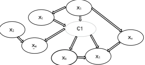
Bayesian networks (BN) are probabilistic graphical models represented by directed acyclic graphs in which nodes are variables (features) and arcs show the relationships among the variables (Castellano, Fanelli, & Pelillo, 1997). The Bayesian network structure S is a directed acyclic graph (DAG) and the nodes in S are in one-to-one correspon-dence with the features X. The arcs represent unintention-al influences among the features while the lack of possible arcs in S indicates conditional independencies. Further-more, a feature node is conditionally independent from its non-descendants given its parents.
-ing Bayesian networks, there exists two scenarios: known structure and unknown structure. In the first case, the struc -ture of the network is given and anticipated to be correct. When the network structure is fixed, learning the parame -ters in the Conditional Probability Tables (CPT) is solved by estimating a locally exponential number of parameters from the given data (Jensen, 1996). Each node in the network has an associated CPT describing the conditional probabil-ity distribution given the different values of nodes’ parents.
Despite the notable power of Bayesian Networks, they have an essential limitation. This is the computational diffi -culty of discovering a previously unknown network. In other scenario, when the structure is unknown, one method is to introduce a scoring function or a score that evaluates the “fitness” of networks with respect to the training data, and then to search for the best network according to this score (Kotsiantis, Zaharakis, & Pintelas, 2007).
Table 1 down explains the training phase for BNs.
Table 1. Steps for training BN
Bayesian Network considers prior information about a given problem, in terms of structural relationships among its features. This prior domain knowledge, about the structure of a BN can take the following forms:
• declaring that a node is a root node, and thus, has no parents;
• declaring that a node is a leaf node and thus, it has no children;
• declaring that a node is a direct cause or direct effect of another node;
• declaring that a node is not directly connected to anoth-er node;
• declaring that two nodes are independent, given a con-dition-set and
• providing partial nodes ordering; that is, declare that a node appears earlier than another node in the ordering.
Fig. 1. Bayesian Network structure sample
Problematic point of BN classifiers is that they are not suitable for datasets with many features. It is due to the reason of not feasible time and space if constructing very large network. Furthermore, before induction process, the numerical features’ discretization is required in most cases (Cheng, Greiner, Kelly, Bell, & Liu, 2002).
Naive Bayes model is technically a special case of Bayesian networks (Lazkano & Sierra, 2003), while Bayes-ian Network represents a set of variables as a graph of nodes and makes inherent assumptions about dependence and independence between those nodes. Naive Bayes as-sumes that all the features are conditionally independent of each other. By taking into consideration the fact that in reality two variables are virtually never independent, Naïve Bayes assumption works well in most cases. Additionally, computation cost and quantity of the data in Bayesian Net-work, often heads to the simplification of the data training process by approximation that variables that are nearly in-dependent are fully inin-dependent as in Naive Bayes model. In our study we use Naive Bayes (NB) classifier as a classification method alone and as a part of the hybrid clas -sifier.
Instance-based learning
Instance-based learning algorithms delay the induction or generalization process until classification is performed, that is why they are known as lazy-learning algorithms (Mitch-ell, 1997). The computation time during the training phase is less than eager-learning algorithms (such as decision trees, neural networks and Bayes networks) (Kotsiantis, Za-harakis, & Pintelas, 2007) but more computation time for the classification process is required. One of the most straight -forward instance-based learning algorithms is the nearest neighbor algorithm. A review of instance-based learning classifiers can be found within these works: (Phyu, 2009 ), (Gent, et al., 2010).
to the query instance and defines its class by detecting the single most frequent class label. In order to achieve bet-ter classification rates, several algorithms use weighting schemes by voting influence of each instance instead of distance measurements between the samples or points x and y. On the other hand, distance can be measured, for in-stance, using Euclidean (Formula 2) or Minkowski Distance (Formula 3):
(2)
Formula 2: Euclidean Distance Measure
(3)
Formula 3: Minkowski Distance Measure
Different distance measurement formulas can also be applied, which are known by names of: Manhattan, Cheby-chev, Camberra or Kendall’s Rank Correlation (Phyu, 2009 ). A review of weighting schemes is given by Wettschereck (Wettschereck, Aha, & Mohri, 1997)
kNN classifier is powerful due to its nonparametric archi -tecture, simplicity and no requirement for training time. But some reservations can be addressed about the algorithm: (i) memory intensiveness, (ii) low speed of classification/ estimation, (iii) sensitiveness to the choice of the similari-ty function used to compare samples, and (iv) the lack of principled way to choose k, as the selected amount of k has an influence on the performance of the kNN algorithm (At -tal, Mohammed, Dedabrishvili, & Chamroukhi, 2015; Elkan, 2011). For instance, a larger k should be selected when noise is present in the locality of the query instance to avoid the incorrect classification caused by the majority vote of the noisy instance (s). Alternatively, a smaller number of k is solution when the region defining the class, or fragment of the class, is so small that instances belonging to the class that surrounds the fragment may win the majority vote.
The major drawback of instance-based algorithms, as already stated above, is their large computational time for classification. Determining the input features (via feature selection) which are intended to be used in modelling pro-cess is a key issue to scale down the required classification time and enhance the algorithm’s performance (Yu & Liu, 2004). Moreover, accuracy of instance-based classifiers can be improved by selecting suitable distance metric for the specific dataset.
Algorithm Combination Methodology
There are various methods suggested for the creation of ensemble of classifiers (Tulyakov, Jaeger, Govindaraju, & Doermann, 2008). Even though one can find number of pro -posed techniques of ensemble creation, there is as yet no clear picture of which technique is finest (Villada & Drissi, 2002). Consequently, construction of good combination of classifiers is an active area of research in supervised learn -ing. There are three main methodologies to build an ensem-ble of classifiers: (i) by means of different subsets of training data with a particular learning technique, (ii) by means of different training parameters with a particular training tech -nique (e.g., using different initial weights) and (iii) by means of different learning techniques. While combining classifiers complementary information can be gained by fusing the dif-ferent sources. All those described combinations can pro-duce appreciable improvements (Lazkano & Sierra, 2003; Sierra, Lazkano, Martinez-Otzeta, & Astigarraga, 2003).
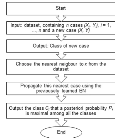
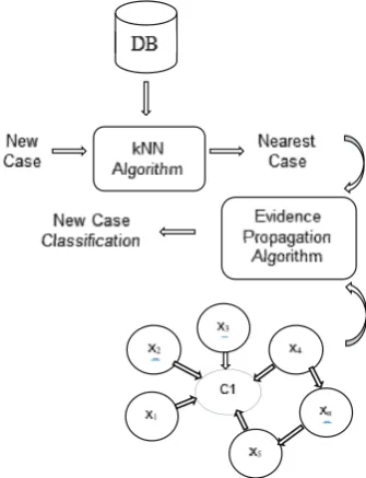
Steps of the combined algorithm is presented in figure 3. New cases in the training dataset are classified according to the nearest case and final decision is made by propagating the evidence of this nearest case in the previously learned Bayesian Network. The schema of the method is shown in Figure 4.
Fig. 4. The scheme of new case classification
Experimental Results
In this section, we will review and compare experimental results on the dataset of human activity recognition using multi-classifier or hybrid classifier of NB and kNN.
While learning the dataset, new cases were classified according to the following process:
(i) Firstly, we looked for the nearest neighbor case in the training database affording to the kNN algorithm, where, Ki represented the nearest case.
(ii) Then, we propagated the Ki case in the learned BN as if it was the new case, (iii) and finally, after propaga -tion according to the posteriori higher probability (which is done by achieving two sub-goals of the Bayesian network approach: fixing the network structure and establishing the values of the probability tables for each node) we marked the new case with class label.
The results of the experiments are given in table 2. As described in previous work, (Attal, Mohammed, Dedabrish-vili, & Chamroukhi, 2015) dataset has passed the prepro-cessing phase and its’ dimensionality is reduced using Prin-cipal Component Analysis.
Table 2. Performance Evaluation of the Algorithms
(%) Accuracy Error Rate Precision Recall kNN 0.99253 0.00747 0.98851 0.98851 NB 0.94286 0.05714 0.94286 0.95887 kNN-NB 0.99526 0.00474 0.99526 0.99527
As shown from the performance evaluation of the algo-rithms, hybrid classifier of kNN and Naive Bayes has the highest accuracy rate compared to separately used clas-sifiers.
Table 3 shows a list of activities performed by humans on everyday basis. Those activities represent different classes in the dataset and are marked by A1 – A12. Reader is directed to previous study (Attal, Mohammed, Dedabrish-vili, & Chamroukhi, 2015) for detailed information about the dataset.
Table 3. List of the selected activities (A1 . . . A12)
Activity Reference Activity Description
A1 Stair Descent
A2 Standing
A3 Sitting Down
A4 Sitting
A5 From sitting to sit on the ground A6 Sitting on the ground
A7 Lying down
A8 Lying
A9 From lying to sit on the ground
A10 Standing up
A11 Walking
A12 Stair ascent
Table 4. Confusion matrix obtained with k-NN Classifier
Predicted Classes
A1 A2 A3 A4 A5 A6 A7 A8 A9 A10 A11 A12
A1 99.00 0.32 0.00 0.00 0.00 0.00 0.00 0.00 0.00 0.08 0.48 0.12 A2 0.06 99.75 0.04 0.00 0.00 0.00 0.00 0.00 0.00 0.03 0.07 0.04 A3 0.00 0.43 99.15 0.43 0.00 0.00 0.00 0.00 0.00 0.00 0.00 0.00 A4 0.00 0.00 0.11 99.79 0.11 0.00 0.00 0.00 0.00 0.00 0.00 0.00 A5 0.00 0.00 0.00 0.23 99.38 0.23 0.00 0.00 0.08 0.08 0.00 0.00 A6 0.00 0.00 0.00 0.00 0.07 99.78 0.07 0.00 0.03 0.05 0.00 0.00 A7 0.00 0.00 0.00 0.00 0.00 0.21 99.65 0.14 0.00 0.00 0.00 0.00 A8 0.00 0.00 0.00 0.00 0.00 0.00 0.15 99.79 0.06 0.00 0.00 0.00 A9 0.00 0.00 0.00 0.00 0.08 0.17 0.00 0.33 99.42 0.00 0.00 0.00 A10 0.35 0.18 0.00 0.00 0.09 0.09 0.00 0.00 0.00 99.20 0.09 0.00 A11 0.22 0.17 0.00 0.00 0.00 0.00 0.00 0.00 0.00 0.00 99.34 0.28 A12 0.08 0.17 0.00 0.00 0.00 0.00 0.00 0.00 0.00 0.04 0.25 99.45
Table 5. Confusion matrix obtained with Naïve Bayesian Classifier
Predicted Classes
A1 A2 A3 A4 A5 A6 A7 A8 A9 A10 A11 A12
A1 100.00 0.00 0.00 0.00 0.00 0.00 0.00 0.00 0.00 0.00 20.00 0.00
A2 0.00 100.00 0.00 0.00 0.00 0.00 0.00 0.00 0.00 0.00 0.00 0.00
A3 0.00 0.00 100.00 0.00 0.00 0.00 0.00 0.00 0.00 0.00 0.00 0.00
A4 0.00 0.00 0.00 100.00 0.00 0.00 0.00 0.00 0.00 0.00 0.00 0.00
A5 0.00 0.00 0.00 0.00 100.00 0.00 0.00 0.00 0.00 0.00 0.00 0.00
A6 0.00 0.00 0.00 0.00 0.00 80.00 0.00 0.00 0.00 0.00 0.00 0.00
A7 0.00 0.00 0.00 0.00 0.00 0.00 100.00 0.00 0.00 0.00 0.00 0.00
A8 0.00 0.00 0.00 0.00 0.00 0.00 0.00 71.43 0.00 0.00 0.00 0.00
A9 0.00 0.00 0.00 0.00 0.00 20.00 0.00 28.57 100.00 0.00 0.00 0.00
A10 0.00 0.00 0.00 0.00 0.00 0.00 0.00 0.00 0.00 100.00 0.00 0.00
A11 0.00 0.00 0.00 0.00 0.00 0.00 0.00 0.00 0.00 0.00 80.00 0.00 A12 0.00 0.00 0.00 0.00 0.00 0.00 0.00 0.00 0.00 0.00 0.00 100.00
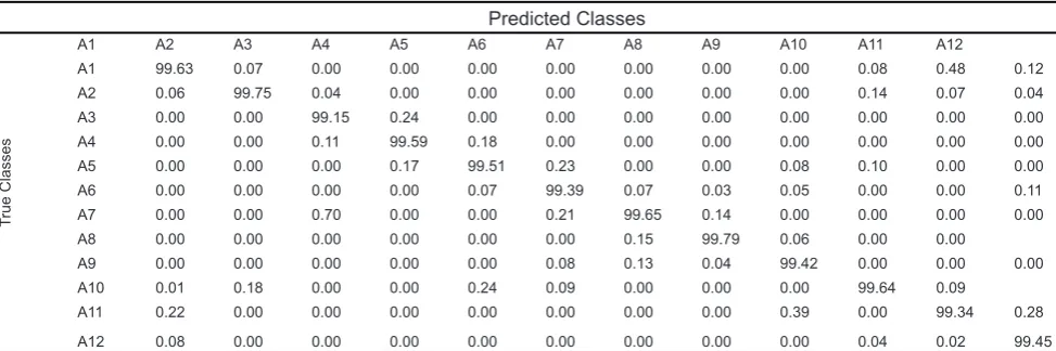
Table 6. Confusion matrix obtained with Hybrid Classifier of k-NN and Naïve Bayesian
Predicted Classes
A1 A2 A3 A4 A5 A6 A7 A8 A9 A10 A11 A12
A1 99.63 0.07 0.00 0.00 0.00 0.00 0.00 0.00 0.00 0.08 0.48 0.12 A2 0.06 99.75 0.04 0.00 0.00 0.00 0.00 0.00 0.00 0.14 0.07 0.04 A3 0.00 0.00 99.15 0.24 0.00 0.00 0.00 0.00 0.00 0.00 0.00 0.00 A4 0.00 0.00 0.11 99.59 0.18 0.00 0.00 0.00 0.00 0.00 0.00 0.00 A5 0.00 0.00 0.00 0.17 99.51 0.23 0.00 0.00 0.08 0.10 0.00 0.00 A6 0.00 0.00 0.00 0.00 0.07 99.39 0.07 0.03 0.05 0.00 0.00 0.11 A7 0.00 0.00 0.70 0.00 0.00 0.21 99.65 0.14 0.00 0.00 0.00 0.00 A8 0.00 0.00 0.00 0.00 0.00 0.00 0.15 99.79 0.06 0.00 0.00 A9 0.00 0.00 0.00 0.00 0.00 0.08 0.13 0.04 99.42 0.00 0.00 0.00 A10 0.01 0.18 0.00 0.00 0.24 0.09 0.00 0.00 0.00 99.64 0.09 A11 0.22 0.00 0.00 0.00 0.00 0.00 0.00 0.00 0.39 0.00 99.34 0.28 A12 0.08 0.00 0.00 0.00 0.00 0.00 0.00 0.00 0.00 0.04 0.02 99.45
True Classes
True Classes
Conclusions
This paper presents the study of the human activity recog-nition dataset using hybrid classifier that combines Bayes -ian Networks with distance-based classifier, namely, with k Nearest Neighbour. The evidence propagation in the Bayesian Network is accomplished for the nearest case in the training database instead of the case that is being classified by the BN algorithm itself. By seeking the nearest case and selecting the class with the maximum a posteriori probability we can decrease the time cost for predicting new case which is essential while developing real-time applica-tions and thus provide better classification accuracy.
Obtained results show that the hybrid of the algorithms outperforms the classification rate of solely used Bayesian Network as well as kNN when this latter is applied as a clas-sifier model.
Presented approach can be extended by grouping of other significant classification techniques in the Supervised or Unsupervised Learning environments. Study of the data-set using different classification algorithms and more im -portantly, using combination of classifiers, as this method provides promising achievements (Vishwakarma & Kapoor, 2015), can point to the construction of good hybrid classifier in terms of performance and accuracy rate which is vital in elderly population’s lives while dealing with activity recog-nition.
References
Attal, F., Mohammed, S., Dedabrishvili, M., & Chamroukhi, F. (2015). Physical Human Activity Recognition Using Wear-able Sensors. Sensors, 31314-31338.
Biau, G., & Devroye, L. (2015). Lectures on the Nearest Neighbor Method (Springer Series in the Data Sciences). Springer.
Castellano, G., Fanelli, A., & Pelillo, M. (1997). An iterative pruning algorithm for feedforward neural networks. iEEE Trans Neural Netw 8:, (pp. 519–531).
Cheng, J., Greiner, R., Kelly, J., Bell, D., & Liu, W. (2002). Learning Bayesian networks from data: an information based approach. Artif Intell 137:43–90.
Cowell, R. G., Dawid, A. P., Lauritzen, S., & and Spiegel-harter, D. J. (1999). Probabilistic Networks and Expert Sys-tems. Springer.
Dasarathy, B. V. (1991). Nearest neighbor (nn) norms: Nn pattern recognition classification techniques. IEEE Comput -er Society Press.
Elkan, C. (2011). Nearest Neighbor Classification.
Gent, I. P., Kotthoff, L., Miguel, I., Moore, N. C., Nightingale, P., & Petrie, K. (2010). Learning When to Use Lazy Learning in Constraint Solving. 873-878.
Jain, A., Murty, M., & Flynn, P. (1999). Data clustering: a review. ACM Comput Surveys 31(3), pp. 264–323.
Jensen. (1996). An introduction to Bayesian networks. Springer.
Jensen, F. V. (1997). Introduction to Bayesian Networks Har/Dskt Edition. Springer.
Kotsiantis, S. B., Zaharakis, I. D., & Pintelas, P. (2007). Machine learning: a review of classification and combining techniques. Springer.
Lazkano, E., & Sierra, B. (2003). BAYES-NEAREST: a new Hybrid classifier Combining Bayesian Network and Dis -tance Based algorithms. Springer.
Li, A., Ji, L., Wang, S., & Wu, J. (2010, November 15-17). Physical activity classification using a single triaxial accel -erometer based on HMM. IET International Conference on Wireless Sensor Network, IET-WSN., pp. pp. 155–160. Mitchell, T. (1997). Machine learning. McGraw Hill.
Pearl, J. (1988). Probabilistic Reasoning in Intelligent Sys-tems: Networks of Plausible Inference. . Morgan Kaufmann. Peterek, T., Penhaker, M., Gajdoš, P., & Dohnálek, P. (2014). Comparison of Classification Algorithms for Phys -ical Activity Recognition. Advances in Intelligent Systems and Computing, vol 237. Springer, Cham.
Phyu, T. N. (2009 ). Survey of Classification Techniques in Data Mining. Proceedings of the International MultiConfer-ence of Engineers and Computer Scientists Vol I IMECS 2009. Hong Kong.
Ruiz, Z., Salvador, J., & Garcia-Rodriguez, J. (2017). A Sur-vey of Machine Learning Methods for Big Data. Springer, Cham. Springer International Publishing AG.
Sierra, B., Lazkano, E., Martinez-Otzeta, J., & Astigarraga, A. (2003). Combining Bayesian Networks, k Nearest Neigh-bours algorithm and Attribute Selection for Gene Expres-sion Data Analysis.
Stiefelhagen, R., & Garofolo, J. (2007). Multimodal Tech-nologies for Perception of Humans: First International Eval-uation Workshop on Classification of Events, Activities and Relationships, ... Papers (Lecture Notes in Computer Sci-ence). Springer Edition.
Tulyakov, S., Jaeger, S., Govindaraju, V., & Doermann, D. (2008). Review of classifier combination methods. Springer. Villada, R., & Drissi, Y. (2002). A perspective view and sur -vey of meta-learning. Artif Intell Rev 18:, 77–95.
Vishwakarma, D., & Kapoor, R. (2015). Hybrid classifier based human activity recognition using the silhouette and cells. Expert Systems with Applications: An International Journal, Volume 42 Issue 20, 6957-6965.