(UDC: 616.281:577.3]:519.87)
A 1D pipe finite element with rigid and deformable walls
M. Kojic1,2,3*, M. Milosevic1 , V. Simic1, M. Ferrari2
1
Belgrade Metropolitan University - Bioengineering Research and Development Center BioIRC Kragujevac, Prvoslava Stojanovica 6, 3400 Kragujevac, Serbia
2 The Methodist Hospital Research Institute, The Department of Nanomedicine, 6670 Bertner Ave., Houston, TX 77030
3 Serbian Academy of Sciences and Arts, Knez Mihailova 35, 11000 Belgrade, Serbia * Corresponding author
Abstract
The authors have formulated a simple 1D finite element for fluid flow and heat or mass transport by diffusion. The element is computationally efficient and suitable for modeling large systems of pipe segments. Motivation for this development came from a need for efficient computational models for mass transport within biological systems, such as blood vessel network, or capillary network within tumors. A detailed derivation of the fundamental equations is presented, with numerical examples which illustrate the element accuracy.
Keywords: 1D finite element, pipe flow, rigid walls, deformable walls, diffusive transport
1. Introduction
Flow of a Newtonian fluid within straight pipes with rigid walls and uniform circular cross-section can be considered as Poiseuille flow, with a parabolic velocity profile. This is true for steady flow conditions, but for transient and oscillatory flows it can be considered as a good approximation. Also, deviation from a parabolic profile occurs for large velocities within small pipe cross-sections and laminar flow, where the profile tends to a flat-shape (details are given below). In case of relatively small wall deformations (diameter change up to the order, say, 10%) the flow could be still considered as in case of rigid pipes.
On the other hand, flow through pipe branching is three-dimensional. Then, 3D models are necessary. The 3D models of branching, in general, require significant effort in the 3D FE mesh generation and are computationally demanding. These models are not suitable for large pipe networks, as in case of blood vessel systems. Therefore, it is desirable to have simpler, efficient, 1D finite elements which can be practically used as a good approximation of the flow within large pipe networks. This approximation is particularly acceptable for modeling of flow within complex capillary networks present in healthy tissue and especially in tumors. These facts have been a motivation to here explore possibility of formulation of 1D pipe FE, and this study has been prepared having in mind capillary networks.
where the network is represented by blood vessel segments with common edges (nodes) within the net. Pressure change along segments is governed by the Hagen-Poiseuille law, while the pressure is equal for all segments at the common node and the total flux at interior nodes is equal to zero. A system of linear equations with respect to nodal pressures is formed and solved with the given boundary conditions - pressures and/or fluxes (Lipowsky et al. 1974, Pries et al. 2009). Our development relies on the same assumptions, but is generalized by including pipes with deformable walls.
The paper is organized as follows. In the next section we present a review of the basic relations for pipe flow, and then in Section 3 we formulate our 1D pipe finite element. In Section 4 are given several examples, and some concluding remarks are presented in Section 5.
2. Fundamental relations for pipe flow
Here we summarize the fundamental relations for flow within deformable pipes, which serve as a basis for the development of the finite element models. We consider axisymmetric flow of viscous incompressible fluid within circular deformable pipe. It is assumed that the pipe is straight, the flow is unsteady and that the fluid is Newtonian. Regarding the fluid-wall interface, a no-slip condition is adopted.
A general concept presented in (Smith et al. 2002, Canic and Kim 2003) will basically be followed to derive the governing equations. Continuity equation in the cylindrical coordinate system can be written as:
0
1
r
rv
r
x
V
x r(1)
where x and r are axial and radial coordinates, and vx and vr are axial and radial fluid velocity
components. The balance of linear momentum in the axial direction, expressed as the Navier-Stokes equation, is:
2 2 2 21
1
x
v
r
v
r
r
v
v
x
p
x
v
v
r
v
v
t
v
x x x xx x r x
(2)where p is fluid pressure, and ρ and
are density and kinematic viscosity, respectively. In pipe flow the term
2v
x/
x
2 can be neglected due to the fact that radial velocities are much smaller that the axial velocities (Canic and Kim 2003). Then (2) can be written as:
r
v
r
r
r
v
x
p
x
v
v
r
v
v
t
v
x xx x r
x
1
1
(3)or in a form suitable for further derivations,
r
v
r
r
v
x
rp
x
rv
v
r
v
rv
t
rv
x xx x r x
1
(4)0
2
2
t
R
R
t
R
R
v
x
v
(5) and0
2
1
2
2
2
2 2
R xr
v
R
v
x
p
x
v
x
v
v
x
R
R
v
t
R
R
v
t
v
(6)where v is the mean velocity of the pipe cross-section,
R xdr
rv
R
v
0 22
(7)and
R xdr
rv
v
R
0 2 2 22
(8)is a dimensionless energy parameter often used in pipe flow (Formaggia et al. 2001 and 2003, Sherwin et al. 2003a, Milisic and Quarteroni 2004, Sherwin et al. 2003b, Sochi 2013). The
derivative x R
v
r
depends on the velocity profile within the pipe, which can be expressed in aform: v R r vx
12 (9)
where
is a parameter depending on the flow character. In case of a parabolic profile which occurs in a fully-developed steady conditions
2
, while for large arteries and pulsatory flow it can be taken
9
(Ref. Hunter 1972 cited in Smith et al. 2002). With given
, the parameter
can be determined from (8) as
2 /
1
; for a parabolic profileα=4/3 With vx expressed by (9), the Navier-Stokes equation (6) can be written as:
0
2
2
1
2
2
2
2 2
R
v
x
p
x
v
v
x
R
R
v
t
R
R
v
t
v
(10)The next fundamental relation which will be used further is related to wall deformation. It is assumed that the wall thickness is small with respect to the radius, hence the wall can be considered as a cylindrical thin shell, so that the axial deformation is negligible (physiologically verified condition for blood vessels) ; and that material is elastic. Under these conditions, the current pipe radius can be expressed in terms of the pressure at the cross-section as follows:
E p R v R R
0 2 0 1 1 where
R
0 is the initial radius,
is the wall thickness (considered constant); and E and
are Young’s modulus and Poisson ratio of the wall material, respectively.We further express continuity equation (5) and balance of linear momentum equation (10) in terms of the cross-sectional mass-flux Q,
v R Av
Q 2
(12)where A is he cross-sectional area. Also, we employ the pipe constitutive relation (11), from which follows:
t
p
R
k
t
R
E
2 (13)where
E R v
kE
0 2
1
(14)
Is the elastic constant. Note that in case of a rigid pipe
k
E
0
, the wall tissue can be considered incompressible, and the elastic constant isk
E
3
R
0/ 4
E
. With use of (12) and (14), the continuity equation (5) can be written as:0
2
3
x
Q
t
p
k
R
g (15)Further, after some straightforward algebra, equation (10) can be obtained in the form of force balance along the pipe axis:
0
2
2
2
1
2
x
p
A
Q
R
x
R
A
Q
R
x
Q
A
Q
t
Q
(16)We note that in case of a rigid pipe, the continuity equation reduces to:
0
x
Q
(17)while (16) becomes:
0
2
2
x
p
A
Q
A
t
Q
(18)In case of steady flow and fully-developed Poiseuille flow (
2
) the balance of forces equation reduces to the well-known Hagen-Poiseuille equation:0
x
p
kQ
(19) where
8
4R
is a pipe characteristic which will be further used in our derivation; the reverse of k represents the viscous resistance to flow, used in literature.
In further development of the 1D finite element for pipe flow, we will use equations (15) and (16) as the fundamental equations, as well as (17) and (19) as their special cases.
3. One-dimensional finite element for flow within deformable pipe
We first derive the basic FE equation of mass balance of our 2-node finite element, then introduce Lagrange multiplier method to enforce continuity at a branching point, and finally formulate equations for 1D diffusion.
3.1. Element formulation
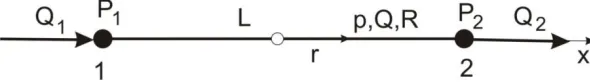
We consider 2-node finite element with data shown in Fig. 1: nodal pressures are P1 and P2, nodal fluxes are Q1 and Q2, while at a position r (where the pipe radius is R) they are p and Q; element length is L.
Fig. 1. Pipe finite element, basic data
In order to derive governing equations for a pipe finite element and general conditions incorporated into fundamental equations of Section 2, we proceed as follows.
Our goal is to develop a finite element with the nodal pressure as the only nodal variable to be determined within an incremental-iterative scheme of the FE assemblage. To achieve this, we differentiate the governing equation (16) with respect to x, to obtain:
0 2
2 4
1 1
2 , 2 , , ,
2
,
xx x xx
x x
p Q R x
R A Q RA
QQ Q
A t
Q
A
(20)where “,x” and “,xx” denote first and second derivative with respect to x. In deriving this
equation we have taken that
/
x
0
, which means that change of the velocity profile along the element is neglected; also, derivative of the cross-section area A is neglected, i.e. it is taken
A
/
x
0
. Next, we further drop-out the second term in (20) as small with respect others, and obtain:
0 2
2 4
1
, ,
,
xx x x
p Q R x
R A Q RA
t Q
A
(21)Before proceeding to derive the finite element balance equation for a general case of deformable pipe and under transient conditions, consider a special case of steady flow through rigid pipe. Then we have constant flux Q (equation (17)), and (21) reduces to:
0
,xx
p
(22)J J
IJ
P
Q
K
(23)where
L
k
K
K
K
K
11
22
12
21
(24)and
Q
Q
Q
1
2
(25)are nodal fluxes with positive sign if the flux is in direction of normal to the cross section. If a pipe network is modeled by this linear pipe element, boundary conditions include prescribed pressures and fluxes, which can be functions of time. Since the system is linear, the system of equations is solved once for a given time, without any trace of history of pressure/fluxes evolution. The FE model is computationally very efficient: there is no numerical integration for evaluation of element matrices and it has one degree of freedom per node. Therefore, the model is suitable for large pipe networks, as in case of capillary beds with huge number of branching. It will be shown in solved examples that distribution of flux among pipe segments with a common junction is according to equation (23), and the net mass flux at the junction is equal to zero, i.e.
0
1
n
i I i
Q
(26)where I is a common node, and n is number of branching segments.
The finite element for a rigid pipe under steady conditions can serve as the basic element and the solutions obtained with deformable pipe and unsteady flow can be considered as perturbed with respect to the basic ones.
We now return to the deformable pipe and equation (21). To eliminate the flux as the nodal variable, we use continuity equation (15) from which it follows:
t
p
k
t
p
k
R
x
Q
g
g
3
2
(27)where
g
g
R
k
k
2
3
(28)and substitute
Q
/
x
into (21). Then, the balance equation (21) can be written in the form:0
, 22 2
1
p p xxkp
t
p
m
t
p
m
(29)
R
x
R
A
Q
RA
k
k
m
A
k
k
m
g p g p2
2
4
2 1
(30)Equation (29) is written in a way to lead to the previously element matrix (24) in case of rigid pipe. This equation represents the equation of balance of linear momentum, with adopted approximations, in terms of pressure only. The coefficients
m
2p, k andk
E are dependent on the current pipe radius and the flux, so that we transform (29) into the incremental-iterative finite element form:
p i JtIJ i J i IJ i p IJ I ext i J i IJ i p
IJ
K
P
Q
M
K
P
M
P
M
1
1
1
1 1
1 (31)where
Q
ext Iis external flux, and:
L x J x I i i IJ L J I i p i p i p IJdx
N
N
k
K
dx
N
N
m
t
m
t
M
, , 1 1 1 2 1 1 11
(32)Here, NI are the interpolation functions along the element,
t
is time step, JtP
is the pressure at start of the time step, and i is the equilibrium iteration counter.As can be seen from the expression for m2 in (30), it is necessary to have the value of flux
Q for each iteration. In order to determine Q we write equation (16) in a weak form:
0
1
vp JIJ Jt J vv IJ J vv
IJ
M
Q
Q
K
P
t
Q
K
(33)where
dL
N
R
x
R
RA
Q
N
A
Q
N
K
dL
N
N
M
L J x J I vv IJ J L I vv IJ
2 ,2
2
2
2
(34)
, vp pv
IJ IJ I J x
L
K
K
AN N
dL
and QJt is the nodal flux at start of the time step; summation is implied for the repeated index J: J=1,2. Now, for a calculated nodal pressures PJ(i)from (31), nodal fluxes can be determined (for a finite element) from (33), as:
J pp IJ Jt vv kJ vv Ik I P K Q M K t
Q 1 1 1
(35)
1
1
,
vv vv vv pp vv vp
IJ IJ IJ IJ Ik kJ
K
K
M
K
K
K
t
with summation on the repeated index k, k=1,2. From the nodal fluxes, the flux Q at integration point is evaluated for the current iteration on P in equation (33) and then substituted in (34) to calculate
m
2p i( 1) .3.2. Use of Lagrange multipliers for branching points
We note here that the fluxes QI from (31) do not satisfy the condition (26), or satisfy it approximately, depending mainly on wall deformability. In order to satisfy the continuity condition (26) we use the Lagrange multiplier concept (Bathe 1996, Liu 2010). A node I with a branching is shown:
Fig. 2. Branching at node I. Lagrange parameter λI is introduced at node I to enforce continuity condition (26). For element e nodal pressures and fluxes are P1, PI and Q1, Q2, respectively.
in Fig. 2. The variational form of the continuity condition (26) can be written as (Liu 201014):
0
1 1 1
1
e i J e pp e IJ I e Jt e vv e kJ vv e Ik i J e pp e IJI K M Q K P
t P
K
(36)where λI is the Lagrange multiplier, and summation goes over all elements with the common
node I. In writing (36), the expression (35) for fluxes of elements e has been used. The terms in the element matrix and nodal vector, corresponding to λI (node I can be first or second element node, hence I can be either 1 or 2) are:
I
on
sum
no
;
2
,
1
,
2
,
1
,
,
2 ,2 ,
J
K
F
J
K
K
K
K
I pp JI J pp IJ J J pp IJ J I
(37)2 1
1
, sum on , : ,
1, 2
e vv e vv e Jtpp J
IJ Ik kJ
I
F
K P
K
M
Q
J k
J k
t
where the element nodal variables include P1, P2, λI. With use of the Lagrange multipliers, the total system of equations is extended for number of nodes with branching, and this extended system is solved over time steps and iterations.
3.3. Diffusion balance equations
The fundamental transport convective-diffusion equation in 1D case is (Kojic et al. 2008):
0
q
x
c
D
x
v
x
c
t
c
(38)
where c is volumetric concentration, D is diffusion coefficient, v is velocity at a cross-section within the element, and q is a source term. Using the Galerkin procedure (Kojic et al. 2008), we obtain the balance of mass equation for the finite element as:
v
JIJ IJ Jt
J IJ v
I ext I J v IJ IJ
IJ
M
C
C
K
K
C
t
Q
Q
C
K
K
M
t
1
1
(39)
where CJ and CJt are nodal concentrations at start and end of time step,
Q
Iextare external mass volumetric fluxes, and matrices and nodal vectorQ
Iv are:IJ I J
L
M
A N N dL
, , IJ I x J x
L
K
A DN
N
dL
, v
IJ I J x V
K
vN N
dV
v
I I
L
Q
A N qdL
Analogous equations can be obtained for heat transfer (details can be seen in Kojic et al. 2008).
4. Examples
Here are presented two examples: 1) Example to assess accuracy of our pipe FE when the walls are rigid, and to compare solutions using the two formulations of the element; also, solution of diffusion with convection within the pipe. 2) Example to show the results in case of branching.
4.1. Straight pipe, several segments
Pressure drop along pipe axis for pipes with rigid walls is given in Fig. 3b. As can be seen from Fig. 3a and 3b, pressure drop is
P
= 32.00 Pa, which is same as the analytic solution:
3
2 2
32 10 g / mm s 5
32
200
/
32
1
mm
L
P
v
mm s
Pa
D
mm
which proves accuracy of the presented model and the developed pipe finite element.
Fig. 3. 1D pipe FE model with rigid walls a) The FE model consists of 10 1D finite elements, with prescribed inlet pressure and outlet velocity, together with the pipe velocity (mean fluid velocity) field and pressure field obtained using FE model; b) Pressure distribution along the
pipe length.
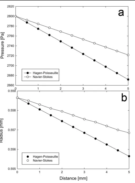
Fig. 4. Fluid flow through 1D pipe elements with deformable walls: Pressure drop (a) and radius change (b) along pipe length for both Hagen-Poiseuille and Navier-Stokes formulations.
Fig. 5. Coupled convective-diffusive transport within pipe with deformable walls. a) Concentration fields at initial, and final time step (t=0.02 s - stationary state). b) Concentration
profiles along pipe length for few different times within transient period (t=0.001, 0.002 and 0.004s) and for stationary state (t = 0.02s)
4.2. Pipe structure with a branching
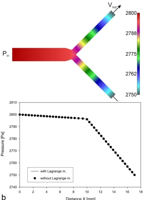
Fig. 6. Pipe structure with branching a) 1D pipe branching model, with pressure field within the segments. b) Pressure profiles along x pipes for both cases, with and without Lagrange
multipliers.
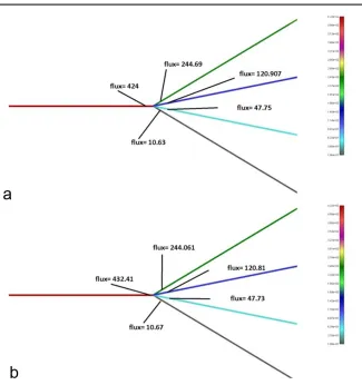
Fig. 7. Pipe structure with branching with four different outlet segments in ratio of 4:3:2:1 (D = 1, 0.75, 0.5, 0.25 respectively). Other data are as in the first example. Element fluxes: a)
solution with Lagrange multipliers, b) solution without Lagrange multipliers
As can be seen from Fig 7, algebraic sum of fluxes in outlet segments (out of branching point) in the method with Lagrange multipliers is Q=423.98 mg/(mm2s), which gives the 0.004% relative error with respect to the flux in inlet segment which is 424 mg/(mm2s).
On the other hand, in case without Lagrange multipliers, algebraic sum of fluxes in outlet segments is Q=423.238 mg/(mm2s), which represents 2.167% relative error with respect to the flux in inlet segment which is 432.41 mg/(mm2s).
5. Concluding remarks
accuracy of both PE and NS formulations. Our finding that use of Lagrange multipliers to enforce continuity conditions at branching, in case of using deformable pipe and the NS formulation, does not significantly contribute to the solution accuracy, and might serve as a useful information for further research in this field.
Acknowledgements
This project has been supported from funds of State of Texas Emerging Technology Fund, Alliance of NanoHealth (ANH), and the Ernest Cockrell Jr. Presidential Distinguished Chair (M.F.)
The authors acknowledge support from Ministry of Education and Science of Serbia, grants OI174028 and III 41007, and City of Kragujevac.
Извод
1Д коначни елемент цеви са крутим и деформабилним зидовима
M. Којић1,2,3*, M. Mилошевић1 , В.Симић1, M. Ferrari2
1
Универзитет Метрополитан Београд – Истраживачко развојни центар за
биоинжењеринг БиоИРЦ Крагујевац, Првослава Стојановица 6, 3400 Крагујевац, Србија 2 The Methodist Hospital Research Institute, The Department of Nanomedicine, 6670 Bertner Ave., Houston, TX 77030
3 Српска Академија Наука и Уметности, Кнез Михаилова 35, 11000 Београд, Србија * аутор за кореспонденцију
Rезиме
Аутори су у овом раду представили једноставан и ефикасан 1Д коначни елемент за спрегнуто струјање течности и провођење топлоте или транспорт масе путем дифузије. Овај коначни елемент је рачунски ефикасан и погодан за моделирање сложених система који се састоје из великог броја сегмената цеви. Мотивација за развој овог елемента је проистекла из потребе за ефикасним рачунским моделима који би се користили за транспорт у сложеним биолошким системима, као што су мрежа крвних судова или капиларна мрежа у тумору. У раду је приказано детаљно извођење основних транспортних једначина, заједно са примерима који показују тачност представљеног 1Д коначног елемента.
Кључне речи: 1D коначни елемент, струјање кроз цеви, крути зидови, деформабилни зидови, дифузиони транспорт
References
Pries, A. R., & Secomb, T. W. Structural adaptation and heterogeneity of normal and tumor microvascular networks. PLoS Computational Biology 5 (2009).
Smith, N. P., Pullan, A. J. & Hunter, P. J. An anatomically based model of transient coronary blood flow in the heart. SIAM J. Appl. Math. 62, 990–1018 (2002).
Canic, S. & Kim, E. H. Mathematical analysis of the quasilinear effects in a hyperbolic model blood flow through compliant axi-symmetric vessels. Math. Meth. Appl. Sci. 26, 1161– 1186 (2003).
Formaggia, L., Gerbeau, J. F., Nobile, F. & Quarteroni, A. On the coupling of 3D and 1D Navier-Stokes equations for flow problems in compliant vessels. Comput. Methods Appl. Mech. Engrg. 191, 561-582 (2001).
Formaggia, L., Lamponi, D. & Quarteroni, A. One-dimensional models for blood flow in arteries. J. Eng. Mathematics 47, 251–276 (2003).
Sherwin, S. J., Franke, V., Peiro, J. & Parker, K. One-dimensional modelling of a vascular network in space-time variables. J. Eng. Mathematics 47, 217–250 (2003a).
Milisic, V. & Quarteroni, A. Analysis of lumped parameter models for blood flow simulations and their relation with 1D models ESAIM: Math. Modelling Num. Analysis 38, 613–632 (2004).
Sherwin, S. J., Franke, V., Peiro, J. & Parker, K. Computational modelling of 1D blood flow with variable mechanical properties and its application to the simulation of wave propagation in the human arterial system. Int. J. Numer. Meth. Fluids 43, 673–700 (2003b). Sochi, T. Comparing Poiseuille with 1D Navier-Stokes flow in rigid and distensible tubes and
networks. (King's College of London, London, 2013).
Hunter, P. J. Numerical solution of arterial blood flow MS thesis, University of Auckland, (1972).
Kojic, M., Filipovic, N., Stojanovic, B. & Kojic, N. Computer Modeling in Bioengineering - Theoretical Background, Examples and Software. (John Wiley and Sons, 2008).
Bathe, K. J. Finite element procedures (Prentice-Hall, Inc., 1996).