Integrated Detection, Tracking and Recognition
for IR Video-based Vehicle Classification
Xue Mei, Shaohua Kevin Zhou
†, Hao Wu, Fatih Porikli
‡University of Maryland †Siemens Corporate Research ‡Mitsubishi Electric Research Labs
College Park, MD 20742 Princeton, NJ 08540 Cambridge, MA 02139
[email protected] [email protected] [email protected]
Abstract— We present an approach for vehicle classification in IR video sequences by integrating detection, tracking and recognition. The method has two steps. First, the moving target is automatically detected using a detection algorithm. Next, we perform simultaneous tracking and recognition using an appearance-model based particle filter. We present a probabilistic algorithm for tracking and recognition that incorporates robust template matching and incremental subspace update. There are two template matching methods used in the tracker: one is robust to small perturbation and the other to background clutter. Each method yields a probability of matching. The templates are represented using mixed probabilities and updated when the appearance models cannot adequately represent the variations in object appearance. We also model the tracking history using a nonlinear subspace described by probabilistic kernel princi-pal components analysis, which provides a third probability. The most-recent tracking result is incrementally integrated into the nonlinear subspace by augmenting the kernel Gram matrix with one row and one column. The product of the three probabilities is defined as the observation likelihood used in a particle filter to derive the tracking and recognition result. The tracking result is evaluated at each frame. Low confidence in tracking performance initiates a new cycle of detection, tracking and classification. We demonstrate the robustness of the proposed method using outdoor IR video sequences.
Index Terms— detection, tracking, recognition, tracking evaluation, IR video
I. INTRODUCTION
Recently, video-based vehicle classification has gained much attention, especially in automatic traffic manage-ment, surveillance and battlefield awareness. Typically, detection and tracking are often solved before classifi-cation. [1] discusses pose determination and recognition of vehicles in traffic scenes, which under normal condi-tions stand on the ground-plane. In [2], a segmentation algorithm uses deformable template models to segment a vehicle of interest both from the stationary complex back-ground and other moving vehicles in an image sequence. In addition to segmentation, the deformable template algorithm also classifies the vehicle of interest. In [3], the author describes a system for automatic recognition
This paper is based on “Integrated Detection, Tracking and Recog-nition for IR Video-based Vehicle Classification,” by X. Mei, S. K. Zhou, and H. Wu, which appeared in the Proceedings of the IEEE International Conference on Acoustics, Speech and Signal Processing (ICASSP), Toulouse, France, May 2006. c°2006 IEEE.
of vehicle type from frontal views. They only use images and it does not involve tracking. In [4], a method for rec-ognizing a vehicle’s maker and model is proposed. It first creates a compressed database of local features of target vehicles from training images and then matches them with the local features of the probe image for recognition. Ma and Grimson [5] proposed a repeatable and discriminative feature to describe a relative large region and the whole set of features forms a rich representation for object classes.
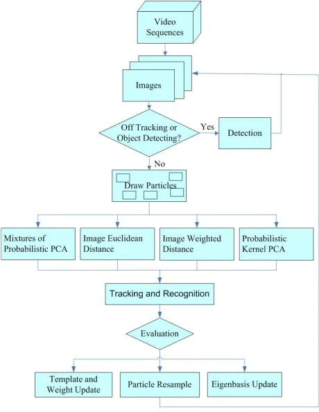
Figure 1. A flow chart of our system.
detected using temporal variance analysis. The target is tracked and classified simultaneously using a robust and adaptive appearance model and mixtures of probabilistic principal component analysis [6](PPCA). Evaluation of the tracking performance is performed at each frame. If the performance falls below some threshold, the cycle of detection, tracking and classification is re-initiated, otherwise the tracking and classification propagates to the next frame. The target-to-background contrast is very low for the IR images. This adds much difficulty for detection and tracking of the moving target. Feature-based classification methods fail due to the insufficient feature points on the detected vehicles.
Unlike Zhou et al. [7]’s method which manually selects the moving target in the first frame, we automatically select it using temporal variance analysis algorithm. Be-cause of the presence of smoke and dust in IR videos, it is hard to position a tight rectangular bounding box from the detection algorithm. Consequently, the tracker drifts quickly. This brings a need for the evaluation of the tracking performance. The evaluation generates a confidence measure to indicate whether we should restart the detection once the tracking confidence falls below a threshold. In [7], Zhou et al. use sum of squared distance(SSD) for the tracked object and template to give the probability of tracking. Therefore, it gives the same weight to each pixel. Here we propose to use two template matching algorithms, Image Euclidean Distance and Image Weighted Distance, to substitute SSD. Both distances assign a weight based on the difference between pixel intensities. These two algorithms are robust to small perturbation and background clutter. Additionally, a third probability pKP CA is provided by the probabilistic kernel Principal Component Analysis(PCA) that models a nonlinear subspace of the tracking history. The com-bination of these separate tracking algorithms has been justified in [8]. After tracking, we update the models to adapt to the most-recent appearance change. For the two template matching methods, the template library is modeled using mixed probabilities. The template with the smallest weight is replaced by the most-recent tracking result when the probability is below some threshold. The weight for each mixture component is updated adaptively. For the nonlinear subspace modeling of tracking history, the most-recent tracking result is added by augmenting the kernel Gram matrix with one more row and column. The standard particle filter algorithm is then used: the samples are re-sampled to eliminate particles with small importance weights and concentrate on particles with large weights. We use mixtures of PPCA [6] for appear-ance modeling. We then compute the posterior probability of finding the appearance of each object in the given video and assign the label corresponding to the maximum. Tracking and classification then proceed to the next frame to repeat the same procedure.
The remainder of the paper is organized as follows. In the next section, we review the particle filter algorithm. Section III briefly describes detection algorithm. Section
IV details the two template matching algorithms and how to update the template library. Section V presents the probabilistic kernel PCA used for modeling the tracking history. Section VI describes the simultaneous tracking and classification algorithm. Section VII describes evalu-ation for the tracking. Experimental results are reported in section VIII. In section IX, we conclude our work.
II. PARTICLEFILTER
The particle filter is a Bayesian sequential importance sampling technique for estimating posterior distribution of state variables characterizing a dynamic system. It consists of essentially two steps: prediction and update. The predicting distribution of xt given all available ob-servations z1:t−1 ={z1, z2,· · ·, zt−1} up to time t−1, denoted by p(xt|z1:t−1), is recursively computed as
p(xt|z1:t−1) =
Z
p(xt|xt−1)p(xt−1|z1:t−1)dxt−1 (1)
At time t, the observation zt is available and the state vector is updated using the Bayes’s rule
p(xt|z1:t) =p(zt|xt)p(xt|z1:t−1)
p(zt|z1:t−1) (2) wherep(zt|xt)denotes the observation likelihood.
In the particle filter, the posterior p(xt|z1:t)is
approx-imated by a finite set of N samples {xi
t}i=1,···,N with
importance weights wi
t. The candidate samples xit are
drawn from an importance distribution q(xt|x1:t−1, z1:t)
and the weights of the samples are updated as
wti=wt−i 1
p(zt|xi
t)p(xit|xit−1)
q(xt|x1:t−1, z1:t) (3)
The samples are resampled to generate a set of equally weighted particles according to their importance weights to avoid degeneracy. In the case of the bootstrap filter
q(xt|x1:t−1, z1:t) =p(xt|xt−1) and the weights become the observation likelihoodp(zt|xt).
III. TARGETDETECTION
Distinguishing foreground objects from the stationary background is both a significant and difficult research problem. Detection plays an important role in our system. It is a prerequisite for tracking and places an initial bounding box around the target and re-initialize the target if tracking confidence measure is low. We adopt temporal variance analysis for object detection. It is effective, easy to implement and can detect moving objects at real-time. In the following, we review the temporal variance analysis for object detection.
Given a video sequences {Ii}, we set m1 = I1 and
mv1=I1×I1. The operator×is the element-by-element product of two matrices. The following mi, mvi and
imvari are defined as
mi = ((N−1)∗mi−1+Ii)/N (4) mvi = ((N−1)∗mvi−1+Ii×Ii)/N (5)
where N is the window size for detection which is 150 in our experiment.mi,mvi andimvari are updated asi
involves.
We apply fix-level threshold to each elementp(i, j)in
imvari
p(i, j) =
½
1 ifp(i, j)> T
0 otherwise
whereT is the threshold which is preset by the user. Now
imvariis converted to a binary image which is dubbed as variance image. We then select the rectangular bounding box for the moving targets by checkingp(i, j) = 1in the image.
IV. TEMPLATEMATCHING
Template tracking was suggested in the computer vision literature in [9] that dates back to 1981. The object is tracked through the video by exacting a template from the first frame and finding the object of interest in successive frames. SSD was used to calculate the distance between the template and the image. It gives the same weight to each pixel and is not robust to small perturbation and background clutter. The template has a specific shape, ellipse or rectangle, which inevitably includes some background pixels if the object is not perfectly in that shape or the tracker does not locate the object precisely. If the background has similar appearance as the object due to the illumination change, low contrast and noise, the appearance model cannot distinguish it from the background and tracking is prone to drift away. A fixed appearance template is not sufficient to handle recently changes in the video, while a rapidly changing model is susceptible to drift. Two approaches have been proposed to overcome the drift problem [10], [11]. In the algorithm proposed in [10], the updated template is aligned with the first template to obtain the final update in order to eliminate drift. In [11], template update is determined by evaluating the error occurring in the next image using the proposed criterion. The method requires no parameters to be adjusted and should be adaptive to deformation at any noise level. Here we propose a robust template matching algorithm that handles small perturbation, background clutter and updating the template.
A. Image Euclidean Distance
Wang et al. [12] propose a new Euclidean distance
for images, which is dubbed as Image Euclidean Dis-tance(IMED). Unlike the traditional Euclidean distance, IMED takes into account the spatial relationships of pixels. Therefore, it is robust to small perturbation. In this section, we summarize their algorithm and detail how it is used in our framework for template matching and derive a probabilistic output from it.
In [12], it has been shown SSD is not a good metric to measure the image distance and a good one should contain the information of pixel distances. If the metric coefficients depend properly on the pixel distances, the computed Euclidean distance is insensitive to small de-formation.
A Euclidean distance between the template and the tracked object is defined as d(x, y) = [(x−y)TG(x− y)]1/2. The metric coefficient gij, where G = (gij), is the Gaussian function, written as
gij=f(|Pi−Pj|) = 1
2πσ2exp{−|Pi−Pj|
2/2σ2} (7)
where Pi and Pj are two pixels, |Pi−Pj| is the pixel distance, and σis the width parameter. We setσ to be 1 in the rest of paper for simplification.
Suppose that two images z and t are rasterized to form two vectors, z = (z1, z2,· · ·, zM N), t =
(t1, t2,· · ·, tM N), where z is the tracking result and t is the template, then the IMED is given by
d2
IM E(z, t) =
1 2π
M NX i,j=1
exp{−|Pi−Pj|2/2}(zi−ti)(zj−tj).
(8) The probability of the presence of the tracked object given the template is written as
pIM E(z|t) =exp{−d2
IM E(z, t)} (9)
which shows that small distance gives high probability.
B. Image Weighted Distance
When we use a rectangle or ellipse to select the region of interest, we inevitably include some background in the region of interest. The background will contaminate the template and contribute to tracking failure. Inspired by [13], we propose an image weighted distance method to overcome this problem.
The image weighted distance is given by
dIM W(z, t) =
M NX i=1
wi(zi−ti)2 (10)
wherewi is the weight assigned to the square difference of each pixel. The weights are smaller for pixels that are farther from the center. Using these weights increases the robustness of matching since the peripheral pixels are the least reliable, being often affected by occlusion, clutter or interference from the background. The weight function is a 2D Gaussian kernel. Suppose w and h are the width and height of the image, respectively. The weight for the pixel at location (x, y)is
w(x, y) = 1−1
2{(
x−x0
w/2 )
2+ (y−y0
h/2 )
2} (11)
where x0 and y0 is the center of the template. The probability of the object being tracked given the template is
pIM W(z|t) =exp{−d2
IM W(z, t)} (12)
C. Template Update
the variations in object appearance due to illumination or pose variations. If we update the template too often, small errors are introduced each time the template is updated. The errors are accumulated and the tracker drifts from the object. We propose an effective template updating strategy which achieves a compromise.
We attempt to overcome the drift problem by introduc-ing a library of templates and usintroduc-ing mixed probabilities. The mixture of Gaussian distributions is used in [14] to simultaneously model and track feature sets and in [15] to model the history intensity of each pixel. The tracking probability for template matching given the template libraryt1:K,p(z|t1:K), is written as
p(z|t1:K) =pIM E(z|t1:K)pIM W(z|t1:K)
={
K
X
k=1
wk∗pIM E(z|tk)} { K
X
k=1
wk∗pIM W(z|tk)} (13)
where K is the number of templates in the library and
wk is the weight assigned to the templatetk.
When the tracker starts working, the template is added to the library when the probability p(z|t1:k) is below
some thresholdp0. After the number of templates in the library reaches the maximum valueK, the template with the smallest weight is replaced by the tracking result whenp(z|t1:k)< p0. The weight of each model increases when the appearance of the tracking object and template is close enough and decreases vice versa. In general, newly-added templates are less reliable than the old ones. The variation in structure and appearance may be due to transient environmental effects. To model the effect of a particular template gaining “trust”, its weight is increased each timep(z|tk)k=1,2,···,K exceeds some threshold. The
increase is at the expense of the other templates. We apply the strategy suggested in [14] to update the weight of the mixture model and the weights are updated as
wif+1=
(
(wif+α) 1
1+α ifp(z|ti)> pi0 wfi 1
1+α otherwise,
(14)
wherepi0is the threshold for templateti,αis the learning rate such thatα∈(0,1), andf is the frame number. The value ofαsets the rate at which component rankings are changed and outmoded representations are removed and “trust” in new representations is gained.
V. INCREMENTALNONLINEARSUBSPACEUPDATE PCA uses a low dimensional space to approximate a high dimensional space, but it restricts itself to a linear setting, where high-order statistical information is discarded. Kernel PCA overcomes this disadvantage by using a ‘kernel trick’. The essential idea of the kernel PCA is to avoid the direct evaluation of the required dot product in a high-dimensional feature space using the kernel function. Hence, no explicit nonlinear mapping function projecting the data from the original space to the feature space is needed. Since a nonlinear function is used, albeit in an implicit fashion, high-order statistical in-formation is captured. Probabilistic PCA [16], [17] gives
a probabilistic output by decomposing the data space into two subspaces, a principle subspace and a residual subspace. Kernel PCA is implemented by mapping the data space to a higher dimensional space using a nonlin-ear function. Probabilistic kernel PCA has demonstrated its advantage over other traditional subspace approaches in face recognition [18]. We propose an approach that analyzes kernel principal components in a probabilistic manner by using probabilistic kernel PCA.
For each frame, we need to update the current eigenba-sis with the tracking result. In [19], [20], the eigenbaeigenba-sis is updated without storing the covariances or the previ-ous training examples using the probabilistic PCA for tracking. We show that when we use probabilistic kernel PCA, the eigenbasis can be incrementally updated very efficiently by augmenting the kernel Gram matrix with one row and column.
Below, we review the probabilistic kernel PCA in [18] and give the details on updating the kernel Gram matrix.
A. Probabilistic Analysis of Kernel Principal Components
Suppose thatx1, x2,· · ·, xN are the given training sam-ples in the original data spaceRq. Kernel PCA operates in
a higher dimensional feature space induced by a nonlinear mapping functionφ:Rq →Rf, wheref > qandf could
even be infinite.
Probabilistic analysis assumes that the data in the feature space follows a special factor analysis model which related an f-dimensional data φ(x) to a latent q -dimensional variable z as
φ(x) =µ+W z+² (15)
where z∼N(0, Iq), ²∼N(0, σ2If), andW is a f ×q loading matrix. Therefore, φ(x)∼N(µ,Σ), where Σ =
W WT +σ2If.
The probability has the form
p(φ(x)) = (2π)−d/2|Σ|−1/2exp{−1
2(φ(x)−µ)
TΣ−1(φ(x)−µ)} (16) The maximum likelihood estimates for µ and W are given by
µ= 1
N N
X
n=1
φ(xn), W=Uq(Λq−σ2Iq)1/2R (17)
whereR is anyq×q orthogonal matrix, andUq andΛq
contain the top q eigenvectors and eigenvalues of theC
matrix, where C = N−1PN
n=1(φn −φ0)(φn −φ0)T, whereφ0=µ, φn =φ(xn).
The MLE forσ2 is approximated as
σ2' 1
f −q{tr(K)−tr(Λq)} (18)
where the(i, j)thentry of the kernel Gram matrixKcan be calculated as follows:
The determinant ofΣis given by
|Σ|=σ2(f−q) q
Y
i=1
λi (20)
whereλi are eigenvalues of the kernel Gram matrixK. Given a vector y ∈ Rq, the Mahalanobis distance L(y) = (φ(y)−µ)TΣ−1(φ(y)−µ) is calculated as follows:
L(y) =σ−2{gy−hTyJQM−1QTJThy} (21)
wheregy andhy are defined by:
gy =k(y, y)−2kyTs+sTKs (22)
hy =ky−Ks (23)
ky= [k(x1, y),· · ·, k(xN, y)]T (24)
s=N−1j (25)
j= [1,1,· · ·,1]T (26)
andJ, QandM are given
J =N−1/2(I−N−1jjT) (27) Q=Vq(Iq−σ2Λ−1)1/2R (28)
M =σ2Iq+WTW (29)
whereVq are eigenvectors of kernel Gram matrixK. There is no explicit nonlinear mapping involved in the calculation. More detailed derivation can be found in [18].
B. Incremental Update of Kernel Gram Matrix
The nonlinear space is divided intoM nonlinear sub-spaces, each subspace modelled by probabilistic kernel PCA. The final probability of the tracking object z is defined as a mixture distribution:
pKP CA(φ(z)) =
M
X
m=1
wm∗pm(φ(z)) (30)
where pm(φ(z))is the probability of kernel PCA in the
mth subspace and wm is the mixture weight. The
most-recent tracking result is added to the subspace which has the maximum probabilitypm(φ(z)). In order to obtain the probability of tracking, we only need to update the kernel Gram matrix K. The kernel Gram matrix is updated as:
Kf+1=
µ
Kf k(x, y) kT(x, y) k(y, y)
¶
(31)
wheref is the index of the frame andx1, x2,· · ·, xn are all the points in the subspace, y is the current tracking result.k(x, y) = (k(x1, y), k(x2, y),· · ·, k(xn, y))T. This requires a lot of storage space because one has to save all the previous tracking results to calculate the kernel Gram matrix. To overcome this problem, we set a limit on the number of samples in each cluster. The oldest sample is discarded to leave the space for the most-recent one. We follow the same strategy used for template matching to update the weights for the subspaces.
VI. TARGETTRACKING ANDCLASSIFICATION This section describes the vehicle tracking and classi-fication algorithm. In section VI-A, the state space model used for tracking and classification is described. Tracking and classification are implemented simultaneously by estimating the posterior distribution . In section VI-B, mixtures of PPCA is briefly described which is used to estimate the distribution of identity variable for the classification.
A. State Space Model
A time series state space model uses the state variable
xt={nt, θt}, which includes identity variablentand 2D affine transformation motion parameters θt. The system equation is written as
nt=nt−1 θt=θt−1+ut, t≥1 (32)
where we assume that the motion variable follows a Markov process with ut as a white Gaussian noise pro-cess. nt ∈ N = {1,2,· · ·, N} indexes the gallery set {I1, I2,· · ·, IN}.
A simple formulation of the observation equation can be characterized as
Zt=T{Yt;θt}=Int+Vt (33)
WhereZtis the image patch of interest in the video frame,
T is an affine transformation to normalize the image to the same size of the gallery images, and Vt is the noise. The observation equation is equivalently characterized by the likelihood p(Yt|nt, θt) = p(Zt|nt). In the next section,
we define p(Zt|nt)as mixtures of PPCA.
The essence of the framework is posterior proba-bility computation, i.e. computing p(nt, θt|Y1:t), whose
marginal posterior probabilityp(nt|Y1:t)solves the
classi-fication task and marginal posterior probabilityp(θt|Y1:t)
solves the tracking task.
Classification is based on a Maximum A Posteriori (MAP) decision rule, namely finding nt that maximizes
p(nt|Y1:t). The Sequential Importance Sampling(SIS)[9]
method is used to approximate and propagate the pos-terior probability p(nt, θt|Y1:t), and marginalization over
variableθtis carried out before applying the classification rule. Detailed descriptions can be found in [7].
B. Mixtures of Probabilistic PCA
Subspace analysis techniques have attracted growing interest in computer vision research. In particular, eigen-vector decomposition has been shown to be an effective tool for solving problems by using low-dimensional vec-tor to represent high-dimensional vecvec-tor. Here we will follow [8] for the mixtures of PPCA.
Given a set of m by n images {Zi}, we form a set of vectors {ti}, where ti ∈ Rd=mn, by lexicographic
ordering of the pixel elements of each imageZi. For any
t in{ti}, we relate it to a corresponding γ-dimensional vector variable xas:
wheredÀγ andµis the mean of thex.
For the case of isotropic noise ε ∼ N(0, σ2I) , the distribution over t-space for a givenxof the form
p(t|x) = (2πσ2)−d/2exp{− 1
2σ2kt−W x−µk 2} (35)
With a Gaussian prior for thex, we obtain the marginal distribution of t
p(t) = (2π)−d/2|C|−1/2exp{−1
2(t−µ)
TC−1(t−µ)}, (36) where the covariance is
C=σ2I+W WT. (37)
The mixtures of PPCA can model more complex data structures. The model parameters are determined using maximum likelihood estimation. The mixture model is defined as:
p(t) =
M
X
i=1
πip(t|i) (38)
where p(t|i) is a single PPCA model and πi is the corresponding mixing proportion, with πi ≥ 0 and
P
πi = 1. Now the three parameters µ, W and σ2 are
associated with each of the M mixture components. We use an iterative EM algorithm for estimation of the model parameters.
VII. TRACKINGEVALUATION
Most practical tracking systems often fail under some situations. This could be either because of illumination changes, pose variation or occlusion. Therefore, the need for automatic performance evaluation emerges in these applications. Fig.2 shows the tracking result after run-ning the tracker for some time. The bounding box is so large that one concludes that the tracker is already failing. Hence, evaluation is necessary to help us terminate tracking and restart the detection-tracking-classification sequence.
Figure 2. The vehicle is off tracking.
Our evaluation algorithm is based on measuring the appearance similarity and tracking uncertainty. The fol-lowing features are examined in our evaluation:
1) Trace complexityqtc: We define the trace complex-ity as the ratio of the curve length and straight length between the target centroids in different frames.
2) Motion step qms: It is defined as the distance between the box centers in two consecutive frames. 3) Scale change qsc: To examine changes in object scale, we use two clues. One is the ratio of the current area to the initial area, the other is the scale change velocity.
4) Shape similarityqss: The change in the aspect ratio of the bounding box is also useful in providing some information about the object shape. It is defined as the ratio of the current aspect ratio over the initial ratio.
5) Appearance change qac: Three measures are used in our algorithm, the first one is the absolute pixel by pixel change between the current frame and the initial frame, the second one is the histogram difference between the current frame and the initial frame and the last one is related to the tracking algorithm over which the proposed algorithm was tested.
To obtain a comprehensive measure of the tracking performance, we combine the above five indicators. We first use empirical thresholds to find whether the tracker is uncertain according to the above five metrics, then we sum the five indicators using different weights to arrive at a confidence measure q. If the sum drops below some threshold, we conclude that the tracking performance is poor and needs re-initialization.
q=X
j∈J
wjI[qj< λj], J ∈ {tc, ms, sc, ss, ac} (39)
where wj and λj are the corresponding weights and thresholds for the evaluation.
VIII. EXPERIMENTS
In this section, we give details of our implemen-tation. Training and testing are described in the next two sections respectively. In our experiment, the vehicle motion is characterized by θ = (a1, a2, a3, a4, tx, ty), where{a1, a2, a3, a4}are the deformation parameters and
(tx, ty) are the 2D translation parameters. By applying an affine transformation using θ as parameters, we crop the region of interest so that it has the same size as the still template in the gallery and perform zero-mean-unit-variance normalization. The region of interest is24×30
in size.
A. Training
We use one video sequence for each vehicle and obtain the tracking result. Then we select 36 images for each vehicle in the gallery. The pertinent parameters for the experiment are M = 2 andγ= 15.
Six vehicles are used in the experiment and there are a total of 216 images in the gallery. After we have the gallery images, we use mixtures of PPCA to estimate the parametersπi,µi,Wi andσ2
B. Testing
For each frame, we get the motion parameters after tracking and cropping out the region of interest from the original image. After performing zero mean and unit variance operation, we use the result to estimate the posterior probabilities of observing each vehicle. We pick the vehicle which has the highest probability as our classification result after normalization. The probabilities propagate to the next frame. In each frame, if the confi-dence measure is below some threshold, the detection will restart 20 frames before the drifting point and tracking and classification will restart too.
Fig. 3 shows the tracking and recognition results for ‘wetting1’ and Fig. 4 is for ‘bmp1’. In Fig. 3, The image on the top is the tracking result for the current frame. We put a bounding box for the vehicle which we are tracking in each frame with a different color for different vehicles. The image on the bottom left is the classification score which is the probability of seeing each vehicle in the video. It shows the result from the first frame to the current frame. The image to the right is the tracking confidence measure which represents the probability of the correct tracking result. We will restart detection and tracking if the measure falls below the threshold of 0.5. The same description applies to Fig. 4.
0 200 400 600 800 0
0.2 0.4 0.6 0.8 1
Frame Index
Recognition Scores
0 200 400 600 800 0
0.2 0.4 0.6 0.8 1
Frame Index
Tracking Confidence
Figure 3. Tracking and recognition results for ‘wetting1’. The results are from frame 1 to 799. The top panel shows the original image and tracking result, the bottom left panel shows the recognition density
p(nt|Y1:t), and the bottom right panel shows the tracking confidence
q.
From Fig. 3, we observe that the recognition result for the ‘wetting1’ is very good because a high probability is associated with ‘wetting’ (dotted blue line) on almost every frame. There are several peaks and valleys for the dotted blue line due to the re-initialization of the tracking and the evaluation probability on the right drops very quickly at corresponding frames. In Fig. 4, for the recognition of ‘bmp1’, it is confused by ‘brdm’ for first half of the sequence. The tracker quickly drifts away after about 40 frames given the initial location. The result becomes stable and correct after 400 frames. After running the whole video sequence, the correct recognition result is quite good. For this situation, we will classify
0 200 400 600 800 1000 0
0.2 0.4 0.6 0.8 1
Frame Index
Recognition Scores
0 200 400 600 800 1000 0
0.2 0.4 0.6 0.8 1
Frame Index
Tracking Confidence
Figure 4. Tracking and recognition results for ‘bmp1’. The results are from frame 1 to 830.
that the vehicle we are tracking is ‘bmp’ which yields the correct result.
We divide the sixty probe video sequences into ten groups. Each group has each of the six different vehicles. The classification results of one group are summarized in Table I. Each number in a row is the recognition percentage of the vehicle. Taking the second row as an example, 93.13% of the whole sequence recognizes the vehicle as ‘m60’, while 1.39% as ‘brdm’, 3.01% as ‘bmp’, 1.07% as ‘akj’ and 1.40% as ’clw’. No frame recognizes it as ‘wetting’. The elements in the diagonal give the correct recognition score for our experiment. The overall accuracy of the recognition is 90.06%. Our experiment results show all the six probe video sequences can be classified correctly using our proposed method.
IX. CONCLUSION
In this paper, we have proposed an approach for ve-hicle classification by integrating detection, tracking and recognition. After the moving target is detected using temporal variance analysis, it is tracked and classified simultaneously using a robust and adaptive appearance model and mixtures of probabilistic principal component analysis. The multiplication of the outputs of two tem-plate matching algorithms and probabilistic kernel PCA yields tracking probability. Evaluation of the tracking performance is performed at each frame. If the perfor-mance falls below some threshold, the cycle of detection, tracking and classification is re-initiated, otherwise the tracking and classification propagates to the next frame. The experiment results prove our method’s robustness and effectiveness. Our approach can be used as a practical and robust system for surveillance or military purpose from the realm of research to practice.
REFERENCES
m60 brdm wetting bmp akj clw m60 93.13% 1.39% 0 3.01% 1.07% 1.40%
brdm 0 86.58% 0 7.41% 5.87% 0.14%
wetting 0 0 95.12% 1.92% 0 2.96%
bmp 0 13.78% 0 82.75% 2.03% 1.44%
akj 4.91% 1.56% 0.23% 3.15% 90.15% 0 clw 3.14% 0.57% 1.28% 2.36% 0 92.65%
TABLE I.
CONFUSION MATRIX FOR VEHICLE CLASSIFICATION EXPERIMENT.
[2] M.-P. D. Jolly, S. Lakshmanan, and A. K. Jain, “Vehicle segmentation and classification using deformable tem-plates,”IEEE Trans. Pattern Anal. Mach. Intell., vol. 18, pp. 293–308, March 1996.
[3] V. Petrovic and T. Cootes, “Vehicle type recognition with match refinement,” International Conference on Pattern Recognition, vol. 3, pp. 95–98, August 2004.
[4] M. Kagesawa, S. Ueno, K. Ikeuchi, and H. Kashiwagi, “Recognizing vehicles in infrared images using imap parallel vision board,” IEEE Transactions on Intelligent Transportation Systems, vol. 2, pp. 10–17, March 2001. [5] X. Ma and W. Grimson, “Edge-based rich representation
for vehicle classification,”IEEE International Conference on Computer Vision, vol. 2, pp. 1185–1192, 2005. [6] M. Tipping and C. Bishop, “Mixtures of probabilistic
princial component analysers,”Neural Computing, vol. 11, pp. 443–482, 1999.
[7] S. Zhou, R. Chellappa, and B. Moghaddam, “Visual track-ing and recognition ustrack-ing appearance-adaptive models in particle filters,”IEEE Transactions on Image Processing, vol. 13, pp. 1057–7149, 2004.
[8] I. Leichter, M. Lindenbaum, and E. Rivlin, “A probabilistic framework for combining tracking algorithms,”Proc. IEEE Conf. on Comp. Vision and Patt. Recog., pp. 445–451, 2004.
[9] B. Lucas and T. Kanade, “An iterative image registration technique with an application to stereo vision,”In Proc. of IJCAI, pp. 674–679, 1981.
[10] I.Matthews, T. Ishikawa, and S. Baker, “The template update problem,”IEEE Trans. Pattern Anal. Mach. Intell., vol. 26, pp. 810–815, 2004.
[11] T. Kaneko and O. Hori, “Feature selection for reliable tracking using template matching,” Proc. IEEE Conf. on Comp. Vision and Patt. Recog., pp. 796–802, 2003. [12] L. Wang, Y. Zhang, and J. Feng, “On the euclidean
distance of images,” IEEE Trans. Pattern Anal. Mach. Intell., vol. 27, pp. 1334–1339, 2005.
[13] D. Comaniciu, V. Ramesh, and P. Meer, “Kernel-based object tracking,”IEEE Trans. Pattern Anal. Mach. Intell., vol. 25, pp. 564–577, 2003.
[14] N. Dowson and R. Bowden, “Simultaneous modeling and tracking (smat) of feature sets,” Proc. IEEE Conf. on Comp. Vision and Patt. Recog., pp. 99–105, 2005. [15] C. Stauffer and W. Grimson, “Learning patterns of activity
using real-time tracking,”IEEE Trans. Pattern Anal. Mach. Intell., vol. 22, pp. 747 – 757, 2000.
[16] B. Moghaddam and A. Pentland, “Probabilistic visual learning for object representation,” IEEE Trans. Pattern Anal. Mach. Intell., vol. 19, pp. 696–710, 1997.
[17] M. Tipping and C. Bishop, “Probabilistic principal com-ponent analysis,” Journal of the Royal Statistical Society, Series B, vol. 61, pp. 611–622, 1999.
[18] S. Zhou, R. Chellappa, and B. Moghaddam, “Intra-personal kernel space for face recognition,” IEEE In-ternational Conference on Automatic Face and Gesture Recognition, pp. 235–240, 2004.
[19] K. Lee and D. Kriegman, “Online learning of probabilistic appearance manifolds for video-based recognition and
tracking,” Proc. IEEE Conf. on Comp. Vision and Patt. Recog., pp. 852–859, 2005.
[20] D. Ross, J. Lim, and M.-H. Yang, “Adaptive probabilistic visual tracking with incremental subspace update,” Euro-pean Conf. on Computer Vision, pp. 470–482, 2004.
Xue Meiis currently a Ph.D. student at University of Maryland, College Park, USA. He received his BS degrees in Electrical Engineering from the University of Science and Technology of China, Hefei, China, in 2002. His research interests include signal/image/video processing, computer vision, pattern recog-nition, and machine learning.
Shaohua Kevin Zhou received the BE degree in electronic engineering from the University of Science and Technology of China, Hefei, China, in 1994, the ME degree in computer engineering from the National University of Singapore in 2000, and the PhD degree in electrical engineering from the University of Maryland at College Park in 2004. He is currently a research scientist at Siemens Corporate Research, Princeton, New Jersey. Dr. Zhou has general research interests in signal/image/video processing, computer vision, pattern recognition, machine learn-ing, and statistical inference and computlearn-ing, with applications to biometrics recognition, medical imaging, surveillance, etc. Over the past four years, he has published more than 40 book chapters and peer-reviewed journal and conference papers on various topics, including face recognition, database-guided medical image analysis, visual tracking and motion analysis, illumination and pose modeling, kernel machine, and boosting method. He is a frequent reviewer for top-rated journals and conferences. He is a member of the IEEE.
Hao Wureceived her B.S. and M.S. degree in electrical engi-neering from University of Science and Technology of China, in 2000 and 2003 respectively. She is currently a Ph.D. student at University of Maryland, College Park. Her research interests include computer vision, pattern recognition and machine learn-ing. She is a student member of the IEEE.