Comparison of Simple Power Analysis Attack Resistant Algorithms for an Elliptic Curve Cryptosystem

Comparison of Simple Power Analysis Attack

Resistant Algorithms for an Elliptic Curve

Cryptosystem

A. Byrne

, N. Meloni

, A. Tisserand

, E.M.Popovici

and W.P.Marnane

∗

_{Dept. of Electrical and Electronic Engineering, University College Cork}

Email:

{

andrewb,liam,francisc

}

@rennes.ucc.ie

†

_{LIRMM, CNRS - Univ. Montpellier 2}

Email:

{

nicolas.meloni,arnaud.tisserand

}

@lirmm.fr

‡

_{Dept. of Microelectronic Engineering, University College Cork}

Email:

{

e.popovici

}

@ucc.ie

Abstract— Side channel attacks such as Simple Power Analy-sis(SPA) attacks provide a new challenge for securing algorithms from an attacker. Algorithms for elliptic curve point scalar multiplication such as the double and add method are prone to these attacks. The protected double and add algorithm provides a simple solution to this problem but is costly in terms of performance. Another class of algorithm for point scalar multi-plication that makes use of special addition chains can be used to protect against SPA attacks. A reconfigurable architecture for a cryptographic processor is presented and a number of algorithms for point multiplication are implemented and compared. These algorithms have a degree of parallism within their operations where a number of multiplications can be executed in parallel. Sophisticated scheduling techniques can exploit this parallelism in order to optimize the performance of the calculation. Post place and route results for the processor are given.

Index Terms— Cryptography, ellitipic curves, side channel attacks, scheduling techniques

I. INTRODUCTION

Elliptic curve cryptography was proposed by Miller[1] and Koblitz[2] in 1985. It provides a means for two hosts to generate a secret key for communication across an insecure channel. The strength of cryptography lies in the difficulty of an encryption schemes inverse operation. Elliptic curve cryptography provides relatively better security per bit than other cryptographic standards such as RSA[3].

Therefore elliptic curve cryptosystems (ECC) consume less memory and hardware resources to implement. The main operation of ECC is point scalar multiplication given an elliptic curveEand a pointP onEthe point[k]P =P+P+. . . P for some given integerk. The basis for the strength of the ECC is the elliptic curve discrete logarithm problem (ECDLP). Given two pointsQandP on an elliptic curveE, find the integerk such thatQ=kP. For a large enough key size, a brute force attack would require too much computing power and time to be feasible[4].

Recently, more effort has been carried out to secure EC point multiplication against side channel attacks[5]. By mon-itoring side-channel information such as the power consump-tion of a device it is possible to recover the secret informaconsump-tion.

Simple power analysis (SPA) attacks function on a single execution of the cryptographic algorithm under attack. By looking at the power trace of the execution it is possible to identify the different functions of the algorithm. Algorithms such as the double-and-add method are prone to these types of attacks.

One simple solution is the protected double and add method[6] but is costly in terms of calculation time. Euclid’s addition chains can provide both a secure and efficient scheme of exponentiation when combined with elliptic curves[7]. However, as will be seen in Section II-C, finding such chains is a complex task. Therefore we examine another class of addition chains using Zeckendorfs representation that are easier to find.

To implement these algorithms effectively scheduling tools were developed to improve the efficiency of the processor and therefore improve the execution time of a specific algorithm. Bertoni et al. [8] applied similar techniques to the Duursma-Lee algorithm in order to find the optimal configuration for the proposed architecture. In this paper we propose a List-Based Scheduling (LBS)[8] approach to optimise the processor. By monitoring several bits of the secret key at a time, point operations can be grouped together to further improve the performance of the processor.

One of the basic arithmetic operations used for ECC is modular multiplication. Several algorithms for modular arith-metic have been proposed and implemented. Montgomery [9] proposed an efficient algorithm for fast multiplication using a series of additions and right shifts. Daly et al. [10] implemented a number of designs for multipliers based on the Montgomery multiplication. The architecture used in this paper uses two carry propagate adders to perform the multi-plication. Fast carry chain logic in the FPGA allows for a fast implementation but for larger field sizes the carry propagation can lead to very long critical path.

elliptic curves used by the algorithms described in Section II. Section IV describes the versatile processor and the scheduling techniques used to generate it. Implementation results are given.

II. POINTSCALARMULTIPLICATION

Given an elliptic curve E and a point P on the curve, the point Q is calculated by point scalar multiplication where the pointP is added to itself k times to get the point[k]P.

Algorithms such as the double and add algorithm, given in Algorithm 1 are used to calculate point multiplication efficiently. The double and add algorithm requires n_k point doubling operations (n_k is the bit length of the key) andw(k) point additions (w(k)is the binary weight of the key).

Algorithm 1: Double and Add Point Scalar Multiplication

input : P ∈E(GF(q)), k=n_i=0k−1k_i2i

output: Q=kP ∈E(GF(q)) Initialise: Q=P;

fori←n_k−2 to 0do

Q= 2Q //Point Doubling (PD); ifk_i= 1 then

Q=Q+P //Point Addition (PA); end

end

A. Side Channel Attacks

In recent years, cryptosystems have come under attack from various forms of side channel attack. Kocher et al.[5] discovered that cryptosystem implementations leak informa-tion which can help an attackers recover secret data. Two techniques for retrieving secret information in this manner are SPA and differential power analysis (DPA). DPA executes the cryptographic algorithm under attack a number of times and uses statistical analysis to determine the secret information[6]. Countermeasures for ECC such as randomisation of the inputs [11] and blinding techniques[12] can be implemented to protect against such attacks.

SPA involves monitoring the power consumption of a single execution of a cryptographic algorithm. Every instruction has a different power consumption, therefore it is possible to retrieve the sequence of instructions during the algorithm execution. For example, the double and add algorithm has two primary operations, point addition and point doubling. Each of these operations produce a different power trace when executed because of the different number of multiplications and additions in each algorithm. Since, the execution of a point addition in the double and add is directly related to the secret key, it is possible to retrieve the secret key by monitoring the power consumption of a single execution of a scalar multiplication. The first successful power analysis attack against an FPGA was done by Ors et al.[13] in which they attacked an elliptic curve processor and retrieved the secret key.

SPA attacks work well on algorithms where the the power consumption can be directly related to the instruction being ex-ecuted. In order to resist SPA attacks, the power consumption

of the instructions executed in a cryptographic algorithm must not be directly related to the secret data. In the double and add method, the branch instruction based on k_i leaks information about the secret key.

B. Protected double and add

In order to protect the double and add algorithm from a SPA attack, the algorithm needs to be modified. In Algorithm 2 the conditional branch has been removed, thus eliminating the relation between the secret key and the power consumption. This modification is at the expense of a point addition for every bit of the key regardless of the binary weight of the key. This method is therefore inefficient given the number of point operations required.

Algorithm 2: SPA resistant Double and Add Point Scalar Multiplication

input : P∈E(GF(q)), k=n_i=0k−1k_i2i

output: Q[0] =kP ∈E(GF(q)) Initialise: Q[0]=P;

fori←n_k−2 to0 do

Q[0] = 2Q[0] //Point Doubling (PD); Q[1] =Q[0] +P //Point Addition (PA); Q[0] =Q[k_i];

end

C. Euclidean Addition Chains

In this section we present the Euclidean addition chains and show how they can be adapted for elliptic curve point scalar multiplication.

Definition 1: An addition chain computing an integerk is given by a sequencev = (v₁, . . . , v_s)where v₁= 1, v_s=k and∀1≤i≤s, v_i=v_i1+v_i2 for somei₁ andi₂lower than i.

Definition 2: An Euclidean addition chain (EAC)

comput-ing an integer k is an addition chain which satisfies v₁ =

1, v₂= 2, v₃=v₂+v₁and∀3≤i≤s−1,ifv_i=v_i−1+v_j for some j < i −1, then v_i+1 = v_i +v_i−1(case 1) or v_i+1=v_i+v_j(case 2).

Case 1 will be called big step (we add the biggest of the two possible numbers to v_i) and case 2 small step (we add the smallest one).

As an example,(1,2,3,4,7,11,15,19,34)is an Euclidean addition chain computing 34. For instance, in step 4 we have computed 4=3+1, thus in step 5 we must add 3 or 1 to 4, in other words from step 4 we can only compute 5=4+1 or 7=4+3. In this example we have chosen to compute 7=4+3 so, at step 6, we can compute 10=7+3 or 11=7+4 etc. Another classical example of EAC is the Fibonacci sequence (1,2,3,5,8,13,21,34)(which is only made of big steps).

Finding such chains is quite simple, it suffices to choose an integer g coprime with k and apply the subtractive form of Euclid’s algorithm.

subtractive form of Euclid’s algorithm:

34−19 = 15 (big step) 19−15 = 4 (small step)

15−4 = 11 (small step) 11−4 = 7 (big step)

7−4 = 3 (big step) 4−3 = 1 (small step) 3−1 = 2

2−1 = 1 1−1 = 0

Reading the first number of each line gives the EAC (1,2,3,4,7,11,15,19,34).

Finally, in order to simplify the writing of the algorithm, we will use the following notation : ifc= (1,2,3, c₄, . . . , c_s) is an EAC then we only consider the chain from c₄ and we replace all the c_i’s by 0 if it has been computed using a big step and by 1 for a small step. For instance

the sequence: (1, 2, 3, 4, 7, 11, 15, 19, 34) will be written: (1, 0, 0, 1, 1, 0)

1) Point Scalar Multiplication: We can now propose an

algorithm performing a point scalar multiplication using a new function, NewADD. The NewADD function works in the following way: letP₁andP₂be two points on the curve then

NewADD(P₁, P₂) returns two points P₁+P₂ and P₁, where P₁+P₂ is calculated by a Point Addition.

Algorithm 3: Euclid-Exp(c, P)

input : P,[2]P, EAC c= (c₄, . . . , c_s)computingk

output: [k]P∈E

(U₁, U₂)←([2]P, P)

fori= 4. . . sdo ifc_i= 0then

(U₁, U₂)←NewADD(U₁, U₂); else

(U₁, U₂)←NewADD(U₂, U₁); end

end

(U₁, U₂)←NewADD(U₁, U₂); return U₁

Example 2: Let us see what happens with the chain c =

(1,0,0,1,1,0)computing 34:

begin ([2]P, P)

c₄= 1 NewADD(P,[2]P) = ([3]P, P) c₅= 0 NewADD([3]P, P) = ([4]P,[3]P) c₆= 0 NewADD([4]P,[3]P) = ([7]P,[4]P) c₇= 1 NewADD([4]P,[7]P) = ([11]P,[4]P) c₈= 1 NewADD([4]P,[11]P) = ([15]P,[4]P) c₉= 0 NewADD([15]P,[4]P) = ([19]P,[15]P)

NewADD([19]P,[15]P) = [34]P

From the algorithm it can be seen that for a point scalar multiplication using addition chains we need only one initial point doubling followed by s−3 point additions. Therefore, the secret key cannot be retrived by monitoring the power consumption of the instructions executed.

2) About Euclid’s Addition Chains Length: At this point

we know that Euclidean addition chains are easy to compute, however finding small chains is a lot more complicated.

We begin with a theorem proved by D. Knuth and A. Yao in 1975 [14].

Theorem 1: LetS(k)denote the average number of steps to compute gcd(k, g)using the subtractive Euclid’s algorithm whengis uniformly distributed in the range1≤g≤k. Then

S(k) = 6π−2(lnk)2+O(logk(log logk)2)

This theorem shows that if, in order to find an EAC for an integer k, we choose an integer g at random, it will return a chain of length about (lnk)2, which is too long to be used with ECC. Indeed, for a 160-bit exponent to be efficient, Algorithm 3 requires chains of length at most 320. The previous theorem tells us that, theoretically, random chains for a 160-bit exponent have a length of 7,000 on average (it is rather 2,500 in practice). Therefore we need to find ways to reduce the length of these chains.

A classic way to limit the length of EAC is to choosegclose to _φk, where φ=1+₂√5 is the golden section. This guarantees that the last steps of the EAC will be big steps. In practice this method allows EAC of an average length of 1,100 to be found.

Considering 160-bit integers, finding EAC of length 320 can be done by checking (on average) about 30 gs. Finding shorter chains is a lot more difficult, as an example finding chains of length 270 requires testing more than 45,000 gs. Such a computation can not be integrated into any exponen-tiation algorithm so, if some offline computations cannot be performed, one should not expect to use EAC whose length is shorter than 320.

D. Zeckendorf Representation

As we have seen in the previous section, short Eu-clidean addition chains are difficult to find. However, if the integer k is a Fibonacci number, an optimal chain is easy to compute. It is simply the Fibonacci sequence (F₀, F₁, F₂, F₃, F₄, F₅, F₆, F₇...) = (0,1,1,2,3,5,8,13...)

Zeckendorf proposed that any positive integer can be computed as the sum of distinct non-consecutive Fibonacci numbers. This sequence of numbers is called the Zeckendorf representation and is written in the form

k= l

i=2

d_iF_i (1)

withd_i∈ {0,1}andd_id_i+1= 0

To construct the Zeckendorf representation for an integer

subtracted from k to give a new value for k. This process is continued until k is equal to zero. If, afterlsteps, k is reduced to zero we obtain the Zeckendorf representation

k=F_n1+...+F_nl (2)

Example 3: Taking the integer k= 17:

13≤k : 13 (F₇)

17−13 = 4 :k= 4

3≤k : 3 (F₄)

4−3 = 1 :k= 1

1≤k : 1 (F₂)

1−1 = 0

Result : (1, 0, 0, 1, 0, 1)

= F₇ + F₄ + F₂

The Zeckendorf representation needs 44% more digits in comparison with the binary method. For instance a 160-bit integer will require around 230 Fibonacci digits. However, the density of 1’s in this representation is lower, about 0.2764. This means that representing a 160-bits integer requires, on average, 80 powers of 2 but only 64 Fibonacci numbers ( 230×0.2764).

1) Point Scalar Multiplication: Using theNewADDfunction described in Section II-C.1 we can perform a point scalar multiplication of two points on an elliptic curve. Algorithm 4 described this operation. The intermediate points U andV are initialised to the pointP. For every bit of the Zeckendorf representation of the key, a Fibonacci step is computed using the NewADD function for the pointU andV. This is simply a point addition as with the double and add and Addition Chains methods. However, if the bit of the key is non-zero an addition step is computed. This involves a Fibonacci step and some extra multiplications to update the intermediate points P andV. These operations are described in the next section.

Algorithm 4: Fibonacci And Add(k, P)

input : P ∈E(K),k=l_i=2d_iF_i; output: [k]P∈E;

(U, V)←(P, P)

fori=l−1. . .2 do ifd_i= 1then

updateP;

(U, .)←NewADD(U, P) (add step); updateV;

end

(U, V)←NewADD(U, V) (Fibonacci step) ; returnU

end

For a n-bit integer, the classical double and add algorithm requires on average 1.5 ×n operations (n doublings and

n

2 additions) and the Fibonacci and add requires 1.83×n

operations (1.44 ×n Fibonacci steps and 0.398 × n add steps). The Addition chains algorithm requires one initial point doubling and 1.98×n point additions. In other words the Fibonacci and add algorithm requires about 23% more operations while the Addition Chains algorithm requires about

29% more operations. However, Section III will show that the point operations for these two algorithms require fewer multiplications than point doubling and point addition for the

double and add algorithm.

III. POINTOPERATIONS

An elliptic curveE(GF(p))over GF(p) is the set of points P = (x, y),x, y∈GF(p)such that

y2+a₁xy+a₃y=x3+a₂x2+a₄x+a₆, a_i∈GF(p) (3)

along with a special point at infinity∂.

Elliptic curves over large prime fields are described using the Weierstrass equation

y2=x3+a₄x+a₆ (4)

where x, y, a₄ anda₆∈GF(p)and4a3₄ + 27a2₆ = 0. Points on the elliptic curve can be represented in Jacobian coordinates which avoids the need for an expensive inversion operation[15]. Converting from affine to projective coordinates is a simple operation,(x, y,1) → (X, Y, Z). Conversion back however requires a number of modular multiplications and inversions, (x, y) ← (_ZX₂,_ZY₃). In Jacobian coordinates, the curve in Equation 4 is given by

Y2 = X3 +a₄XZ4 + a₆Z6 (5)

A. EC Point Addition(PA) and Doubling(PD)

Consider two separate points on an elliptic curve, P =

(x_p, y_p) and Q = (q_t, q_t). A line l is drawn through the pointsPandQ. The linelintersects the curve at a third point. Q= (x_q, y_q)is the inverse of that point, whereQ=P+Q.

The point addition formula for the curve defined in Equation 4 using Jacobian coordinates are given in Algorithm 5. The computational cost of a point addition is 15 multiplications and 7 add/subs.

Algorithm 5: Point Addition in Jacobian Coordinates input : P(X₁, Y₁, Z₁), Q(X₂, Y₂, Z₂)∈GF(q)

output: P+Q(X₃, Y₃, Z₃)∈E(GF(q))

A = X₁Z₂2, B = X₂Z₁2, C = Y₁Z₂3, D = Y₂Z₁3; E = B − A, F = D − C;

X₃ = −E3 − 2AE2 + F;

Y₃ = −CE3 + F(AE2 − X₃), Z₃ = Z₁Z₂E

If T =P then this is point doubling and a tangent to the point is used. The tangent intersects with the curve at a second point,T= 2(T)is the inverse of this point. Algorithm 6 gives the formulae for point doubling for the curve in Equation 4. The computational cost for point doubling is 10 multiplications and 8 add/subs.

Algorithm 6: Point Doubling in Jacobian Coordinates

input : P(X₁, Y₁, Z₁)∈GF(q)

output: [2]P(X₃, Y₃, Z₃)∈E(GF(q)) A = 4X₁Y₁2, B = 3X₁2 + a₄Z₁4; X₃ = −2A + B2;

B. Reduced Point Addition

Given the formulae in Algorithm 5 and the points P₁ =

(X₁, Y₁, Z) and P₂ = (X₂, Y₂, Z) on the curve E over GF(p), p >3. Then forP₁+P₂=P₃= (X₃, Y₃, Z₃)

X₃ = (Y₂Z3−Y₁Z3)2−(X₂Z2−X₁Z2)3 −2X₁Z2(X₂Z2−X₁Z2)2

= ((Y₂−Y₁)2−(X₂−X₁)3−2X₁(X₂−X₁)2)Z6

= ((Y₂−Y₁)2−(X₁+X₂)(X₂−X₁)2)Z6

= X₃Z6

Y₃ = −Y₁Z3(X₂Z2−X₁Z2)3

+(Y₂Z3−Y₁Z3)(X₁Z2(X₂Z2−X₁Z2)2−X₃)

= (−Y₁(X₂−X₁)3

+(Y₂−Y₁)(X₁(X₂−X₁)2−X₃))Z9

= Y₃Z9

Z₃ = Z2(X₂Z2−X₁Z2)

= Z(X₂−X₁)Z3

= Z₃Z3

Thus we have (X₃, Y₃, Z₃) = (X₃Z6, Y₃Z9, Z₃Z3) ∼

(X₃, Y₃, Z₃).

So when P₁ andP₂ have the same z-coordinate,P₁+P₂ can be obtained using the following formulae:

Algorithm 7: Point Addition, P and Q sharing same Z coordinate

input : P(X₁, Y₁, Z), Q(X₂, Y₂, Z)∈GF(q)

output: P+Q(X₃, Y₃, Z₃)∈E(GF(q))

A= (X₂−X₁)2, B =X₁A, C=X₂A, D= (Y₂−Y₁)2,; X₃ = D − B − C,;

Y₃ = (Y₂ − Y₁)(B − X₃) − Y₁(C − B),; Z₃ = Z(X₂ − X₁)

This addition involves 5 multiplications, 2 squarings and 7 additions/subtractions. This formula is quite efficient in terms of computational cost (more than a doubling) but cannot be used with the classic double and add algorithms and require specific exponentiation schemes. They are well suited for use with addition chains and with the Zeckendorf representation scheme (Fibonacci step).

As they require special conditions, these formulae are logically more efficient than any general or mixed addition formulae. Compared to the 15 multiplications and 7 addi-tions/subtractions for point addition in Algorithm 5 this is a great saving.

Some cryptographic protocols only require thex-coordinate of the point [k]P. In this case it is possible to save one multiplication by step of Algorithm 3 by noticing thatZ does not appear during the computation ofX₃ andY₃, thus it is not necessary to computeZ₃ during the process. Thex-coordinate can be recovered at the end.

C. Add Step

Implementing a point scalar multiplication using Zeck-endorf’s representation requires a new point operation, the Add step. The new point addition formula sharing thez-coordinate described in III-B can be used for the Fibonacci step. For the Add step however we first need to compute U +P so the Add step returns U +P andV with the same z-coordinate. Let us suppose thatU = (X_U, Y_U, Z),V = (X_V, Y_V, Z)and P = (x, y,1). First we compute the pointP= (xZ2, yZ3, Z) so that we can computeU+P = (X_U+P, Y_U+P, Z_U+P)using

NewADD. Computing the pointPrequires an extra 3 multipli-cations and a squaring. From our point addition in Algorithm 7 we have thez-coordinate,Z_U+P = (X_U−xZ2)Z. We also have the values(X_U−xZ2)2and(X_U−xZ2)3(AandC−B in Algorithm 7). Using these values, updating the pointV to (X_V(X_U−xZ2)2, Y_V(X_U−xZ2)3, Z(X_U−xZ2))requires only 2 multiplications. The total computational cost of an add step is 10 multiplications and 3 squarings.

When compared to the 5 multiplications, 2 squarings re-quired for a Fibonacci step in Algorithm 4 we see that a SPA attack would be possible. By monitoring the power consumption of Algorithm 4 it would be possible to distinguish between a Fibonacci step and an Add step and hence it would be possible to determine the secret key. A solution for this is to introduce ”dummy” multiplication stages to the shorter Fibonacci step so that the power consumption of the two steps will match. This is very costly but in Section IV-C we will see that by applying some scheduling techniques this cost can be reduced.

IV. ELLIPTICCURVEPROCESSOR

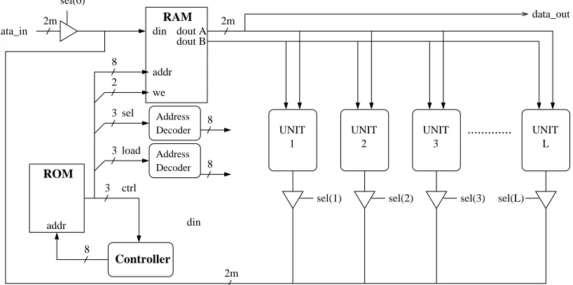
A generic architecture (Figure 1) was designed for cryp-tographic operations which incorporates RAM, a ROM con-troller and a number of arithmetic units for a given field. Software was developed using C++ to generate the VHDL for a customized processor for any characteristic p and extension field m. Everything from the size of the RAM block to config-uring the arithmetic units and generating the ROM instruction set for a given algorithm is controlled by the program.

For prime characteristic fields there is a choice of arithmetic units to chose from for the architecture. Through manipulation of the ROM instructions alone, the processor can be configured for various algorithms including the double and add algorithm or exponentiation using addition chains. In this way, we can quickly compare these and other cryptographic algorithms. The structure of the ROM instructions is explained in Section IV-B while the scheduling required to efficiently implement different algorithms is described in Section IV-C.

A. Arithmetic Units

8

Controller

addr

ROM

dout A dout B

sel(1) sel(2)

...

data_out sel(0)

data_in din

sel(L) sel(3)

din

RAM

we 2

8

addr

8

1 UNIT

2 UNIT

L UNIT 3

UNIT

2m 2m

8

2m ctrl

3 load 3

Decoder Address Decoder Address sel

3

Fig. 1. General Elliptic Curve Processor

The processor architecture in Figure 1 is capable of con-trolling a number of arithmetic units. There are two archi-tecture types available for the GF(p) processor. Dedicated units for each of addition, subtraction and multiplication can be implemented. The number of multipliers implemented in the processor can be configured based on the speed/area constraints of the target technology and the application of the design. Since addition and subtraction only take 4 clock cycles to complete, two of which are RAM read/writes, these operations are best performed in series and do not gain from an increased number of arithmetic units. Alternatively, we can use configurable arithmetic logic units (ALU) that can be set to perform modular addition, subtraction or multiplication. The increased functionality of the units reduces the area consumption compared to the three dedicated units combined. As with the dedicated multipliers, the number of ALUs can be changed to give optimum results based on the target device constraints.

1) Multiplication: In 1985 Montgomery[9] proposed an

efficient method for performing modular multiplication using a series of additions and right shifts. This method avoids the need for costly trial division of the modulus. The Montgomery modular product is defined in Equation 6.

Res = M ont(A, B, p) = AB2−pb+2_{(mod p) (6)}

The output of a Montgomery multiplication is a factor 2−pb+2 _{times smaller than the desired result, p}

b is the field size in bits. In order to correct the result, the output must be Montgomery multiplied by(22pb+2_{mod p})_{. When a large}

number of multiplications are required it becomes inefficient to correct every result. A better solution is to initially convert the numbers to the Montgomery domain. To do this, the number is Montgomery multiplied by (22pb+2 _{mod p})_{. To convert a} number back, it is Montgomery multiplied by 1.

The algorithm for the Montgomery multiplication is given in Algorithm 8. The number of iterations performed isp_b+ 2

in order to the bound the output in the range [0,2p−1] for multiplicands up to twice the modulus. This allows it to be used as an input to further multiplications without the need for conditional subtraction.

Algorithm 8: Montgomery Multiplication

input : A = pb

i=0ai2i, B = ip=0b bi2i,; M = pb

i=0pi2i

output: R = AB2−pb+2(_{mod p})

Initialise:R←0; b_pb+1←0; fori←0 to p_b+ 1 do

q_i = R_i−1 + b_iA(mod2); R_i = (R_i−1 + q_iM + b_iA)/2; end

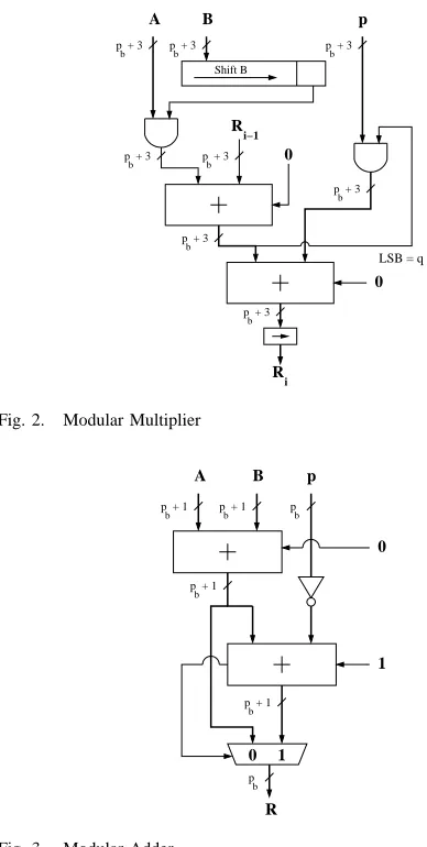
A hardware implementation of the Montgomery multiplier can be seen in Fig. 2. Multiplication is performed according to Algorithm 8. The inputs to the first adder areb_iAand the previous resultR_i−1.q_ipis added to the sum of the first adder if the LSB of the sum (q_i) is equal to 1. A shift register scans each bit ofB forb_iAand the final result is right shift divided by 2.

2) Modular Addition and Subtraction: The modular

addi-tion operaaddi-tion addsA and B in the first adder and subtracts the modulus p from the sum. To subtract the modulus from the intermediate result, the modulus is bitwise inverted and added to(A+B)with the carry-in set to 1, thus performing a two’s complement subtraction. The carry-out of the second adder controls which intermediate result is the correct result. If (A+B)is in the correct range, the result of the first adder is the correct result. Otherwise, the result from the second adder is correct. The architecture for the adder/subtractor in Fig. 3 is configured for modular addition.

b p + 3 Shift B

0

0

i

LSB = q

i−1

R

p B

A

b p + 3 b

p + 3

b

p + 3

b p + 3

i

R

b p + 3 b

p + 3 b p + 3

Fig. 2. Modular Multiplier

0 1

0

1

A B

R p

p + 1 b p + 1b

p + 1 b

p + 1 b

p b

p b

Fig. 3. Modular Adder

must be added to give an output in the correct range.

B. ROM Instruction Set

The processor is controlled by a set of instructions in Xilinx BlockROM and a simple state machine. A similar approach was taken by Leong et al.[17] which helped reduce the development time of the processor and increased the flexibility of the design. A major advantage of this is that the instruction set can be updated to perform any number of operations without the need to recompile the entire processor.

For the field p,plarge prime, dedicated units for modular addition, subtraction and multiplication based on [18] were im-plemented. An example instruction set for the processor over GF(p) using projective coordinates is shown in Table I. After initially loading the elliptic curve parameters and Montgomery constants into RAM, the controller performs operations for the selected cryptographic algorithm. Algorithms such as Point Doubling and Point Addition for the double and add algorithm are stored in ROM. Depending on the current bit of the key, the controller will start at the correct address in ROM.

The 12 LSBs control read and write access to RAM. Bits 12→14 control the tri-states connected to the outputs of the arithmetic units. Only one of these is set high when writing

Instruction Set

ctrl load sel we addr A & B 00 000 000 00 00001 00010 01 011 000 00 00000 00000 00 000 011 01 00000 00011

TABLE I

EXAMPLE INSTRUCTION SET USING DEDICATED ARITHMETIC UNITS

data to RAM. To reduce the impact of a large number of arithmetic units in the design on the size of ROM, a 3-to-8 address decoder is used to make full use of all combinations of the three select bits. Bits 15→17 are the load bits which are used to load new vectors to a specific arithmetic unit. The two MSBs are extra control bits for the state machine controlling the processor.

Some operations such as addition & subtraction execute in a few clock cycles and have no extra timing requirements associated with them. Multiplication however takes p_b + 3 clocks. The MSBs of the instructions are used to trigger delay states in the controller while a multiplication is being performed.

C. Scheduling Methodology

There is a trade off between speed and area that is affected by the number of multipliers implemented in the processor. More multipliers will reduce execution time but will increase the area consumption of the device. To be truly reconfigurable an automated scheduling tool must be used to ensure an efficient implementation. The efficient transfer and processing of data through the processor can greatly improve speed/area tradeoffs.

Two simple methodologies, As-Soon-As-Possible (ASAP) and As-Late-As-Possible (ALAP)[19] assume limitless re-sources and schedule operations either at the earliest or latest time step possible. Given the the lack of constraints the scheduling results are poor and can lead to an inefficient use of resources. More advanced scheduling algorithms such as List-Based Scheduling [8] can efficiently schedule a set of instructions given a set of resource constraints. With LBS we can limit the resources available to the processor and schedule operations for a given algorithm efficiently based on these constraints.

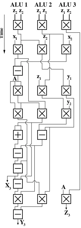
A LBS approach was applied to the various algorithms for a number of different multipliers. Figures 4 and 5 illustrate the schedules generated for algorithms 5 and 6 respectively using three multipliers. The 15 multiplications for a point addition can be executed in five multiplication stages using three multipliers. Similarly, the 10 multiplications for a point doubling can be executed in 5 multiplication stages for the same configuration. Additions and subtractions are performed by separate adders and subtractors.

ALU 1

z₂ z₁z1 z1z2

x₁ z2 x2

y₁ z₁

y2 2

z

A

A

Time

X

Y

Z

3

3 3

ALU 2 ALU 3

Fig. 4. Schedule for Point Addition using three multipliers

share the samez-coordinate requires the fewest multiplications and can be calculated much faster than the other algorithms. The Add Step also has fewer multiplications than the regular point addition but for three multipliers, the regular point addition is actually faster due to the structure of the schedule.

Double & Add Add Chains Fibonacci & Add

Mults PA PD PA (share z) Add Step

1 15pb+ 103 10pb+ 102 7pb+ 63 13pb+ 93 2 8pb+ 82 6pb+ 90 4pb+ 54 7pb+ 75 3 5p_b+ 73 5p_b+ 87 3p_b+ 51 6p_b+ 72

TABLE II

EXECUTION TIME IN TERMS OF CLOCK CYCLES

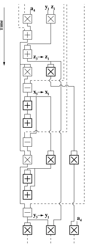
1) Grouping Point Operations: As is evident from Fig. 5,

there are cases where not every multiplier is active for a mul-tiplication stage. For a point doubling using three multipliers, only 10 out a possible 15 multipliers are active. This means during a point doubling the efficiency of the processor is 66%. A solution for this is to combine a number of stages of an algorithm to maximise the efficiency of the processor.

Take for example the double and add algorithm. Looking at two bits of the key at a time we can group a point addition

Time

1 x1

z₁ z₁

x₁ x₁ y₁ y₁

a₄ y1z1

Z3

X3

Y₃

x

Fig. 5. Schedule for Point Doubling using three multipliers

with a point doubling or group two point doublings together, depending on the bits. Table III lists the actions for each combination. Processing two bits at time requires some extra logic for the processor controller.

key Action

00 PD-PD, shift 2 bits 01 PD, shift 1 bit 10 PD-PA, shift 1 bit 11 PD-PA, shift 1 bit

TABLE III

COMBINATIONS FOR POINT OPERATIONS GROUPED IN TWOS

now being used for operations from the second point doubling. The newly active multipliers are highlighted in the figure. The efficiency of the processor for a PD-PD is increased to 83% compared to 66% when performing the point doublings sep-arately. The overall efficiency for the processor implementing the double and add algorithm using three multipliers is 77% with no grouping and 85% when point operations are grouped in twos. It is clear that combining point operations has a positive effect on the performance of the processor.

Time

4 y1z1

a4

y₃ y₁ z₃ z₁

x₃ x₁ a

Fig. 6. Schedule for combined Point Doubling & Point Doubling using three ALUs

A step further is to group the operations in threes. This is done in the same manner as for grouping in twos but instead of monitoring two bits of the key, the controller needs to monitor

three bits. Table IV lists the possible combinations for three bits of the key. This process can be applied for however many bits you want the controller to handle at a time.

key Action

000 PD-PD-PD, shift 3 bits

001 PD, shift 1 bit

01X PD-PD-PA, shift 2 bits 10X PD-PA-PD, shift 2 bits 11X PD-PA, shift 1 bit

TABLE IV

COMBINATIONS FOR POINT OPERATIONS GROUPED IN THREES

D. Scheduling Results

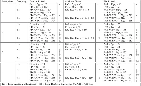
Table V lists the optimum execution times in terms of clock cycles for each algorithm described in the previous sections. The number of multipliers and the level of operation grouping is varied to get an indication of which implementation gives the best performance. It is clear from the table that increasing the number of multipliers reduces the number of multiplication stages required and hence reduces the overall calculation time. Grouping the point operations together also improves the execution time but without the need for extra hardware. The effects of the grouping is marked in the border to the right of the grouped point operations in terms of multiplication stages. The biggest improvement found was for the double and add algorithm using four multipliers. Here, the operations grouped in threes reduced execution time for a number of combinations of the key by four multiplication stages. For example, a PD using four multipliers executes in five multiplication stages. To perform three PDs in series would take 15 multiplication stages. By grouping the three PDs together the number of stages needed is reduced to 11. This improvement is confirmed in Table VII where the execution time of the double and add algorithm using four multipliers is reduced by 1.27ms (25.6%) when operations are grouped in threes.

The architecture presented in Section IV was evaluated on Xilinx xc2v6000-4. The post place and route results for point multiplication using each of the algorithms described in this paper are listed in Tables VI and VII. Each design consumes approximately 5% of the Block RAMs available. The results are based on a 160-bit key size with p_b = 192. This key is used for the double and add and the protected double and

add algorithms. For the addition chains, a chain of length

320 was used while the Zeckendorf representation requires a 230-bit key. We recall however that the binary weight of this representation is about 0.2764. For a 230-bit key this mean we have 64 non-zero digits.

Multipliers Grouping Double & Add Addition Chains Fib & Add

1’s PA = 15p_b+ 103 - PA2 = 7p_b+ 63 - Add = 13p_b+ 93

-PD = 10p_b+ 102 - PD = 10p_b+ 102 - PA2 = 7p_b+ 63

-2’s PD-PD = 20p_b+ 204 - PA2-PA2 = 14p_b+ 126 - PA2-PA2 = 14p_b+ 126

-1 PD-PA = 25p_b+ 205 - Add-PA2 = 20p_b+ 156

-PD-PD-PD = 30p_b+ 306 - Add-PA2-PA2 = 27p_b+ 219

-3’s PD-PD-PA = 35pb+ 307 - PA2-PA2-PA2 = 21pb+ 189 - PA2-PA2-PA2 = 21pb+ 189

-PD-PA-PD = 35p_b+ 307 - PA2-Add-PA2 = 27p_b+ 219

-1’s PA = 8p_b+ 82 - PA2 = 4p_b+ 54 - Add = 7p_b+ 75

-PD = 6pb+ 90 - PD = 6pb+ 90 - PA2 = 4pb+ 54

-2’s PD-PD = 10p_b+ 174 ↑2 PA2-PA2 = 7p_b+ 105 ↑1 PA2-PA2 = 7p_b+ 105 ↑1

2 PD-PA = 13pb+ 189 ↑1 Add-PA2 = 11pb+ 129

-PD-PD-PD = 16p_b+ 264 ↑2 Add-PA2-PA2 = 14p_b+ 180 ↑1

3’s PD-PD-PA = 18p_b+ 256 ↑2 PA2-PA2-PA2 = 11p_b+ 159 ↑1 PA2-PA2-PA2 = 11p_b+ 154 ↑1

PD-PA-PD = 18p_b+ 256 ↑2 PA2-Add-PA2 = 15p_b+ 183

-1’s PA = 5p_b+ 73 - PA2 = 3p_b+ 51 - Add = 6p_b+ 72

-PD = 5p_b+ 87 - PD = 5p_b+ 87 - PA2 = 3p_b+ 51

-2’s PD-PD = 8p_b+ 168 ↑2 PA2-PA2 = 5p_b+ 99 ↑1 PA2-PA2 = 5p_b+ 87 ↑1

3 PD-PA = 9p_b+ 157 ↑1 Add-PA2 = 8p_b+ 120 ↑1

PD-PD-PD = 12pb+ 252 ↑3 Add-PA2-PA2 = 10pb+ 168 ↑2

3’s PD-PD-PA = 12p_b+ 238 ↑3 PA2-PA2-PA2 = 9p_b+ 153 - PA2-PA2-PA2 = 9p_b+ 153

-PD-PA-PD = 14pb+ 244 ↑1 PA2-Add-PA2 = 10pb+ 168 ↑2

1’s PA = 5pb+ 73 - PA2 = 3pb+ 51 - Add = 5pb+ 69

-PD = 5p_b+ 87 - PD = 5p_b+ 87 - PA2 = 3p_b+ 51

-2’s PD-PD = 8pb+ 164 ↑2 PA2-PA2 = 5pb+ 99 ↑1 PA2-PA2 = 5pb+ 87 ↑1

4 PD-PA = 8p_b+ 154 ↑2 Add-PA2 = 7p_b+ 117 ↑1

PD-PD-PD = 11p_b+ 249 ↑4 Add-PA2-PA2 = 9p_b+ 165 ↑2

3’s PD-PD-PA = 11p_b+ 235 ↑4 PA2-PA2-PA2 = 8p_b+ 150 ↑1 PA2-PA2-PA2 = 8p_b+ 150 ↑1

PD-PA-PD = 11p_b+ 235 ↑4 PA2-Add-PA2 = 8p_b+ 162 ↑2

PA = Point Addition (Algorithm 5); PD = Point Doubling (Algorithm 6); Add = Add Step PA2 = Point Addition sharing z-coordinate (Algorithm 7)/Fibonacci Step

TABLE V

EXECUTION TIMES IN TERMS OF CLOCK CYCLES

poorer than the classic double and add algorithm. This is due to the extra point additions require to secure the algorithm from a simple power analysis attack.

The addition chains provided the same security but also perform better than the double and add algorithm. Compared to the double and add algorithm, there is not much gain in grouping point operations for the addition chains algorithm. There is only a slight improvement for grouping operations in pairs and we see a degradation in performance when group in threes. This is due to the structure of the point addition algorithm sharing the z-coordinate. We would expect an improvement in performance for grouping this operation in fours but the logic for the controller would become more complex as four bits would need to be monitored at a time.

It is also worth noting that we see a decrease in calculation time for the protected double and add algorithm when we group point operations in threes for three multipliers. Based on this, it is clear that increasing the level of grouping does not necessarily improve the performance for all algorithms.

In order for the Fibonacci and Add algorithm to be pro-tected against SPA attacks, the power consumption of an execution of the different operations and grouped operations must match. This means that extra multiplications, additions and subtractions must be added to some of the operations. For a configuration with one multiplier this is quite costly as the difference between the add and Fibonacci steps is seven multiplication stages. Even when four multipliers are implemented the added expense of two multiplications for every Fibonacci step to match an Add step inceases the

computation time by over 40%.

However, if we look at the grouped operations in threes for four multipliers, the difference between the grouped operations is a single multiplication stage. For all the operations to match we add extra dummy additions and multiplications to each of the algorithms. The new operations now all execute in 9p_b+ 187clock cycles. For a 160-bit key generating a 230-bit chain with p_b = 192, a point scalar multiplication executes in 4.2ms. This is slower than the Addition Chains method but still outperforms the protected double and add algorithm for the same configuration. Also, as explained in Section II-C finding chains in the Zeckendorf form is much easier than regular addition chains.

V. CONCLUSIONS

In this paper, a reconfigurable cryptographic processor has been used to efficiently compare a number of algorithms for elliptic curve point multiplication. Two algorithms making use of addition chains have been shown to outperform a double

and add approach and provide a solution to SPA attacks.

By varying the number of arithmetic units implemented in the architecture, the processor can be configured for devices with different levels of resources. Also, by grouping point operations for the algorithms we have shown that a gain in calculation time can be achieved. In particular, for the double

and add algorithm using four multipliers we have reduced the

Protected Double and Add Addition Chains

Multipliers 1 2 3 4 1 2 3 4

Slices 2,306 (6%) 2,803 (8%) 3,493 (10%) 3,989 (11%) 2,306 (6%) 2,803 (8%) 3,493 (10%) 3,989 (11%)

min. period (ns) 19.86 19.861 19.809 19.957 19.86 19.861 19.809 19.957

Clock Freq. 50.352Mhz 50.35Mhz 50.35Mhz 50.11Mhz 50.352Mhz 50.35Mhz 50.35Mhz 50.11Mhz

1’s 15.9 9.08 6.61 6.64 8.95 5.23 3.99 4.01

Time (ms) 2’s 15.9 8.53 5.99 5.39 8.95 4.61 3.37 3.39

3’s 15.9 8.46 6.29 5.39 8.95 4.82 3.99 3.59

TABLE VI

POSTPLACE ANDROUTE RESULTS FORXILINX XC2V6000-4

Double and Add Fibonacci and Add

Multipliers 1 2 3 4 1 2 3 4

Slices 2,306 (6%) 2,803 (8%) 3,493 (10%) 3,989 (11%) 2,306 (6%) 2,803 (8%) 3,493 (10%) 3,989 (11%)

min. period (ns) 19.86 19.861 19.809 19.957 19.86 19.861 19.809 19.957

Clock Freq. 50.352Mhz 50.35Mhz 50.35Mhz 50.11Mhz 50.352Mhz 50.35Mhz 50.35Mhz 50.11Mhz

1’s 11.16 6.51 4.96 4.96 9.72 5.56 4.42 4.13

Time (ms) 2’s 11.16 6.03 4.44 4.15 9.72 5.28 3.88 3.65

3’s 11.16 5.71 4.24 3.69 9.72 5.33 3.96 3.48

TABLE VII

POSTPLACE ANDROUTE RESULTS FORXILINX XC2V6000-4

VI. ACKNOWLEDGMENT

The support of the Informatics Commercialisation initia-tive of Enterprise Ireland and Ulysses ”The France-Ireland Exchange Scheme” are gratefully acknowledged

REFERENCES

[1] V. Miller, “Use of Elliptic Curves in Cryptography,” CRYPTO ’85, vol. 218 of Lecture Notes in Computer Science, pp. 417–426, 1986. [2] N. Koblitz, “Elliptic curve cryptosystems,” Math. Computat., vol. 48,

pp. 203–209, 1987.

[3] S. Vanstone, “ECC Holds Key to Next-Gen Cryptography,” Technical

Report, Certicom Corporation, 2004.

[4] N. Koblitz, A. Menezes, and S. Vanstone, “The State of Elliptic Curve Cryptography,” Design Codes and Cryptography, vol. 19, pp. 173–193, 2000.

[5] P. Kocher, J. Jaffe, and B. Jun, “Differential power analysis,” Advances

in Cryptology - CRYPTO’99, vol. 1666 of Lecture Notes in Computer

Science, pp. 388–397, 1999.

[6] J. S. Coron, “Resistance Against Differential Power Analysis for Elliptic Curve Cryptosystems,” Cryptographic Hardware and Embedded Systems

- CHES, vol. 1717 of Lecture Notes in Computer Science, pp. 292–302,

1999.

[7] N. Meloni, “Fast and secure elliptic curve scalar multiplication over prime fields using special addition chains.” Cryptology ePrint Archive, Report 2006/216, 2006. http://eprint.iacr.org/.

[8] G.Bertoni, L.Breveglieri, P.Fragneto, and G.Pelosi, “Parallel Hardware Architectures for the Cryptographic Tate Pairing,” Third Internation

Conference on Information Technology: New Generations, pp. 186–191,

2006.

[9] P.L.Montgomery, “Modular multiplication without trial division,”

Math-ematics of Computations, vol. 44, pp. 519–521, 1985.

[10] A. Daly and W. Marnane, “Efficient architectures for implementing montgomery modular multiplication and rsa modular exponentiation on reconfigurable logic,” International Symposium on Field Programmable

Gate Arrays, pp. 40–49, 2002.

[11] M. Joye and C. Tymen, “Protections Against Differential Analysis for Elliptic Curve Cryptography: An Algebraic Approach,” Cryptographic

Hardware and Embedded Systems - CHES, vol. 2162 of Lecture Notes

in Computer Science, pp. 337–390, 2001.

[12] T. Messerges, E. Dabbish, and R. Sloan, “Power Analysis Attacks of Modular Exponentiation in Smartcards,” Cryptographic Hardware and

Embedded Systems - CHES, vol. 1717 of Lecture Notes in Computer

Science, pp. 144–157, 1999.

[13] S.B.Ors, E.Oswald, and B.Preneel, “Power-analysis attacks on an FPGA - First experimental results,” Cryptographic Hardware and Embedded

Systems - CHES, vol. 2279 of Lecture Notes in Computer Science,

pp. 35–50, 2003.

[14] D. Knuth and A. Yao, “Analysis of the subtractive algorithm for greatest common divisors,” Proc. Nat. Acad. Sct, vol. 72, no. 12, pp. 4720–4722, 1975.

[15] A.Daly, W. Marnane, and E. Popovici, “Fast Modular Inversion in the Montgomery Domain on Reconfigurable Logic,” Irish Signals and

Systems Conference, vol. 19, pp. 363–367, 2003.

[16] A. Daly, W. Marnane, T. Kerins, and E. Popovici, “An FPGA Im-plementation of a GF(p) ALU for Encryption Processors,” Elsevier

Journal on Microprocessors and Microsystems (Special Issue on FP-GAs:Applications and Designs), vol. 28, no. 5-6, pp. 253–260, 2005.

[17] P. Leong and I. Leung, “A Microcoded Elliptic Curve Processor Using FPGA Technology,” IEEE Trans. on VLSI Systems, vol. 10, no. 5, pp. 550–559, 2002.

[18] F. Crowe, A. Daly, and W. Marnane, “A Scalable Dual Mode Arithmetic Unit for Public Key Cryptosystems,” IEEE International Conference on

Information Technology: Coding and Computing (ITCC), vol. 1, pp. 568

– 573, 2005.

[19] K. Parhi, VLSI Digital Signal Processing Systems: Design and