© Universiti Tun Hussein Onn Malaysia Publisher’s Office
IJIE
Journal homepage: http://penerbit.uthm.edu.my/ojs/index.php/ijie ISSN : 2229-838X e-ISSN : 2600-7916
The International
Journal of
Integrated
Engineering
Asymptotic Computational Fluid Dynamic (ACFD) Study of
Three-Dimensional Turning Diffuser Performance by Varying
Angle of Turn
Tham Wei Xian
1, Normayati Nordin
1*, Azian Hariri
1, Nurul Fitriah Nasir
1,
Norasikin Mat Isa
1, Musli Nizam Yahya
1, Suzairin Md. Seri
11Centre for Energy and Industrial Environment Studies, Faculty of Mechanical and Manufacturing Engineering,
Universiti Tun Hussein Onn Malaysia, 86400 Parit Raja, Johor, Malaysia
DOI: https://doi.org/10.30880/ijie.2019.11.05.015
Received 5 March 2019; Accepted 26 March 2019; Available online 10 August 2019
1. Introduction
A diffuser is a device shaped to decelerate fluid. The main goal of a diffuser is to recover the static pressure of the fluid stream meanwhile reducing its flow velocity. Turning diffuser is often introduced in application such as heating, ventilation, air-conditioning (HVAC) system as an adapter to join the conduits of different cross-sectional areas or an ejector to decelerate the flow and raise the static pressure before discharging to the atmosphere [1 - 3]. A diffuser that is introduced with no turn is known as a straight diffuser, whereas a diffuser introduced with certain angle of turn is called a turning diffuser or a curved diffuser [1, 3]. In fluid analysis, outlet pressure recovery coefficient, Cp and flow uniformity
index, σout are basically used to measure the performances of the diffusers. Asymptotic Computational Fluid Dynamics
(ACFD) is the technique combining the asymptotic analysis with Computational Fluid Dynamics that could provide a relationship between dependent and independent variables [1, 5].
The main problem in achieving high recovery is the flow separation which results in non-uniform flow distribution and excessive losses [4, 5]. The geometrical curve shape of turning diffuser will reduce the pressure recovery and flow uniformity and hence the diffuser performance is decreased [5 - 7]. Flow separation occurs when fluid is forced to flow
Abstract: The main problem in achieving high recovery for a tuning diffuser is flow separation which results in
non-uniform flow distribution and excessive losses. Angle of turn is found to affect notably the performance of turning diffuser which its relationship is still unclear particularly for a 3-D case. The present work aims to numerically investigate the effect of varying turning angle, ø = 30° - 180° on the performance of 3-D turning diffuser and to develop the performance correlations via integrating the turning angle using Asymptotic Computational Fluid Dynamics (ACFD) technique. Among all the turbulence models examined, the best validated results were obtained with the Reynold Stress Model with enhanced wall treatment of 𝑦+=1.0 was applied for the intensive simulation. As
the turning angle increased from 30˚ to 180˚, the pressure recovery was reduced by 89.3% and the flow uniformity index was raised by 27.7%. Minimal flow separation took place at 0.75𝐿𝑖𝑛⁄𝑊1 of 90˚ turning diffuser whereas
maximum flow separation happened at 0.44𝐿𝑖𝑛⁄𝑊1 of 180˚ turning diffuser. The performance correlations of 3-D
turning diffuser as a function of geometrical and operating parameters was successfully developed using ACFD method. The ACFD results were kept within ±11.4% of deviation when compared with both CFD and experimental results.
Keywords: Turning diffuser, pressure recovery, flow uniformity, Asymptotic Computational Fluid Dynamics
over a curved surface, the boundary layer no longer attaches to the wall surface and separates from the surface [8, 9]. Researchers found that performance of diffusers were greatly affected by turning angle [10, 11].
Currently, there are available performance correlations of the effect of turning angle on 2-D turning diffuser had been integrated [4]. However, the performance correlations of turning angle on 3-D turning diffuser has not been developed. Therefore, this study aims to investigate numerically the performance of 3-D turning diffuser at various angle (30˚, 90˚, 120˚, 150˚, 180˚) and to develop performance correlations of 3-D turning diffuser via integrating angle of turn.
2.
Methodology
2.1
Performance Index
The performance of diffuser is primarily evaluated by means of:
(i) Pressure recovery coefficient (𝐶𝑝)
𝐶𝑝=
2(𝑃𝑜𝑢𝑡𝑙𝑒𝑡−𝑃𝑖𝑛𝑙𝑒𝑡)
𝜌𝑉𝑖𝑛𝑙𝑒𝑡2 (1)
Where,
𝑃𝑜𝑢𝑡𝑙𝑒𝑡 = average static pressure at diffuser outlet (Pa) 𝑃𝑖𝑛𝑙𝑒𝑡 = average static pressure at diffuser inlet (Pa)
𝜌 = density of air (kg/𝑚3)
𝑉𝑖𝑛𝑙𝑒𝑡 = mean velocity of inlet air (m/s)
(ii) Flow uniformity index, (𝜎𝑜𝑢𝑡)
𝜎𝑜𝑢𝑡= √
1
𝑁−1∑ (𝑉𝑖− 𝑉𝑜𝑢𝑡) 2 𝑁
𝑖=1 (2)
Where,
N = number of measurement points
𝑉𝑖 = local outlet air velocity (m/s)
𝑉𝑜𝑢𝑡 = mean outlet air velocity (m/s)
2.2
Modelling
Turning diffusers with different angle of turn, ø=30˚, 90 ˚, 120 ˚, 150 ˚, and 180 ˚ were modeled as in Fig. 1.
(a) 30˚ turning diffuser (b) 90˚ turning diffuser (c) 120˚ turning diffuser
(d) 150˚ turning diffuser (d) 180˚ turning diffuser
(a) 30˚, (b) 90˚, (c) 120˚, (d) 150˚, (e) 180˚
2.3
Meshing
In this study, hexahedral mesh with skewness less than 0.3 was applied by enabling multizone method. Enhanced wall treatment was applied due to Re < 106 and there was near wall characteristics that needed to be resolved. The
wall-adjacent cell centroid was placed within the viscous sublayer, 𝑦+≈ 1.0. As the inlet velocity was equal to 14.25 m/s,
the corresponding first grid point off the wall was located at 2.8 × 10⁻⁶ 𝑚. The grid independency study was conducted
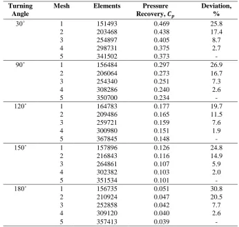
by increasing mesh elements in each step. The simulations were run on different number of elements and the pressure recovery, 𝐶𝑝 was used as reference parameter to determine the convergence of the mesh size. As presented in Table 1,
Mesh 4 provides the least deviation of Cp relative to the finest Mesh 5 in every case thus was chosen as an optimum mesh
to be adopted in the intensive simulation.
Table 1- Mesh independency check for 3D turning diffuser at varying angle
Turning Angle
Mesh Elements Pressure
Recovery, 𝑪𝒑
Deviation, %
30˚ 1 151493 0.469 25.8
2 203468 0.438 17.4
3 254897 0.405 8.7
4 298731 0.375 2.7
5 341502 0.373 -
90˚ 1 156484 0.297 26.9
2 206064 0.273 16.7
3 254340 0.251 7.3
4 308286 0.240 2.6
5 350700 0.234 -
120˚ 1 164783 0.177 19.7
2 209486 0.165 11.5
3 259721 0.159 7.6
4 300980 0.151 1.9
5 367845 0.148 -
150˚ 1 157896 0.126 24.8
2 216843 0.116 14.9
3 264861 0.107 5.9
4 302382 0.103 2.0
5 351534 0.101 -
180˚ 1 156735 0.051 30.8
2 210924 0.047 20.5
3 252858 0.042 7.7
4 309120 0.040 2.6
5 357413 0.039 -
2.4
Governing Equations
The flow was assumed 3-dimensional, steady state and fully developed with negligible gravitational effect. The Reynolds-Averaged Navier-Stokes equations (RANS) as following were solved:
Continuity equation:
𝜕𝑢
𝜕𝑥+ 𝜕𝑣
𝜕𝑦+ 𝜕𝑤
𝜕𝑧 = 0 (3)
x-momentum equation:
𝑢𝜕𝑢
𝜕𝑥+ 𝑣 𝜕𝑢 𝜕𝑦+ 𝑤
𝜕𝑢 𝜕𝑧= −
1 𝜌
𝜕𝑃
𝜕𝑥+ 𝑣 [
𝜕2𝑢 𝜕𝑥2+
𝜕2𝑢 𝜕𝑦2+
𝜕2𝑢 𝜕𝑧2] +
1 𝜌[
𝜕(−𝜌𝑢̅̅̅̅̅̅′2)
𝜕𝑥 +
𝜕(−𝜌𝑢̅̅̅̅̅̅̅̅′𝑣′)
𝜕𝑦 +
𝜕(−𝜌𝑢̅̅̅̅̅̅̅̅′𝑤′)
𝜕𝑧 ] (4)
𝑢𝜕𝑣 𝜕𝑥+ 𝑣 𝜕𝑣 𝜕𝑦+ 𝑤 𝜕𝑣 𝜕𝑧= − 1 𝜌 𝜕𝑃 𝜕𝑦+ 𝑣 [
𝜕2𝑣 𝜕𝑥2+
𝜕2𝑣 𝜕𝑦2+
𝜕2𝑣 𝜕𝑧2] +
1 𝜌[
𝜕(−𝜌𝑢̅̅̅̅̅̅̅̅′𝑣′)
𝜕𝑥 +
𝜕(−𝜌𝑣̅̅̅̅̅̅′2)
𝜕𝑦 +
𝜕(−𝜌𝑣̅̅̅̅̅̅̅̅′𝑤′)
𝜕𝑧 ] (5)
z-momentum equation: 𝑢𝜕𝑤 𝜕𝑥+ 𝑣 𝜕𝑤 𝜕𝑦+ 𝑤 𝜕𝑤 𝜕𝑧 = − 1 𝜌 𝜕𝑃 𝜕𝑧+ 𝑣 [
𝜕2𝑤
𝜕𝑥2+
𝜕2𝑤
𝜕𝑦2 +
𝜕2𝑤
𝜕𝑧2] +
1 𝜌[ 𝜕(−𝜌𝑢̅̅̅̅̅̅̅̅′𝑤′) 𝜕𝑥 + 𝜕(−𝜌𝑣̅̅̅̅̅̅̅̅′𝑤′) 𝜕𝑦 +
𝜕(−𝜌𝑤̅̅̅̅̅̅̅′2)
𝜕𝑧 ] (6)
The applicability of standard k-ε (std k-ε), shear stress transport k-ω (SST k-ω) and Reynolds stress model (RSM) to close the RANS equations was verified. In present work, pressure-based solver was used to solve the governing equations. Each equation was solved separately in pressure-based solver. SIMPLE algorithm, a robust pressure-velocity coupling algorithm which combine the momentum equation and continuity equation that takes the form of pressure correction equation was applied [12, 13]. The gradient was discretised by Green-Gauss-Cell based. Second order scheme was employed for all terms.
2.5
Boundary Conditions
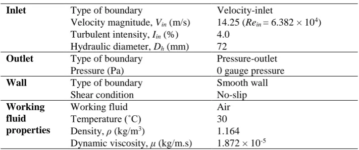
Table 2 shows the boundary operating conditions used during the simulation. At the solid wall, the velocity was zero due to the no-slip condition. The inlet velocity, Vinrespective to the Rein = 6.382 x 10⁴ was specified at 14.25 m/s. This
corresponded to the turbulent intensity, Iinof 4.0%. At the outlet boundary, the pressure was set at the atmospheric
pressure (0 gage pressure). The working fluid was air at 30°C with ρ = 1.164 kg/m3 and μ = 1.872 x 10⁻⁵ kg/m.s.
Table 2- Boundary operating conditions
Inlet Type of boundary Velocity-inlet
Velocity magnitude, Vin (m/s) 14.25 (Rein = 6.382 × 10⁴)
Turbulent intensity, Iin (%) 4.0
Hydraulic diameter, Dh (mm) 72
Outlet Type of boundary Pressure-outlet
Pressure (Pa) 0 gauge pressure
Wall Type of boundary Smooth wall
Shear condition No-slip
Working fluid properties
Working fluid Air
Temperature (˚C) 30
Density, ρ (kg/m3) 1.164
Dynamic viscosity, μ (kg/m.s) 1.872 × 10⁻⁵
2.6
ACFD Method
In this study, effects of geometrical and operational parameters (𝑅𝑒𝑖𝑛, W2/W1, Lin/W1, X2/X1, ø) were correlated with
performance of turning diffuser (𝐶𝑝,𝜎𝑜𝑢𝑡) by using ACFD method. The steps in ACFD technique to develop correlations
of performance or turning diffuser included:
1. Identifying the dependent and independent variables
2. Linearizing the relationship between the dependent and independent variables 3. Applying the Taylor’s series expansion
4. Determining the convergence point and gradients 5. Substituting all the constants to complete the correlations
Cp 3DTD acfd = f (Rein, W2/W1, Lin/W1, X2/X1, ø) (7)
𝜎𝑜𝑢𝑡 3DTD acfd = f (Rein, W2/W1, Lin/W1, X2/X1, ø) (8)
Applying Taylor’s series expansion as below:
η (ϕ1, ϕ2, ϕ3, … ϕn) = ηref + (ϕ1 - ϕ1 ref)
𝜕𝜂
𝜕𝜙1 + (ϕ2 – ϕ2 ref) 𝜕𝜂
𝜕𝜙2 + (ϕ3 – ϕ3 ref) 𝜕𝜂
𝜕𝜙3 + … + (ϕn – ϕn ref) 𝜕𝜂
𝜕𝜙𝑛 (9)
η = dependent variables (Cp, 𝜎𝑜𝑢𝑡)
Dimensionless independent groups:
a, b, c, d and e were selected to make all lines could intersect and converge at one point in graph.
ηref= reference value of dependent variable (intersection/convergence point at y-axis)
ϕ ref = reference value of dimensionless groups (intersection/convergence point at x-axis)
∂η
∂ϕ = gradients/slopes of the corresponding lines
3.
Results and Discussions
3.1
CFD Validation Results
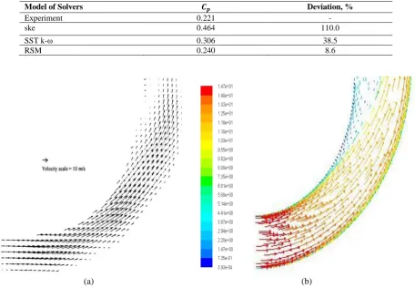
The pressure recovery generated using RSM solver model gave the smallest deviation. Standard k-ε model and stress transport k-ω model created relatively higher deviation of results. After the validation was conducted in different aspects, RSM was selected as the most suitable solver model among 3 chosen models to deal with the 3-D turning diffuser case. The ability of RSM model to exhibit the pattern of 3-D flow and examine high swirly flow had given it advantage to deal with current work. The deviation of 𝐶𝑝 from different solver models with the experimental result was tabulated in Table
3. The comparison of flow structures between the experimental result and RSM model solver was shown in Fig. 2.
Table 3- Deviation of 𝑪𝒑 of different model of solvers
Model of Solvers 𝑪𝒑 Deviation, %
Experiment 0.221 -
ske 0.464 110.0
SST k-ω 0.306 38.5
RSM 0.240 8.6
(a) (b)
Fig. 2- Flow structures, (a) Flow structure [1], (b) Flow structure of RSM
ϕ1 = [
𝑅𝑒𝑖𝑛
𝑅𝑒𝑖𝑛 𝑟𝑒𝑓] 𝑎
ϕ2 = [
𝐿𝑖𝑛 𝑊1 𝐿𝑖𝑛 𝑊1𝑟𝑒𝑓
] 𝑏
ϕ3 = [
𝑊2 𝑊1 𝑊2 𝑊1𝑟𝑒𝑓
] 𝑐
ϕ4 = [
𝑋2 𝑋1 𝑋2 𝑋1𝑟𝑒𝑓
] 𝑑
ϕ5 = [
Ø
3.2
Effect of turning angle, ø
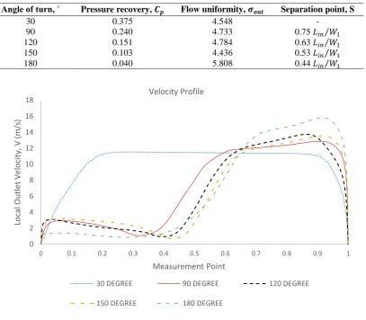
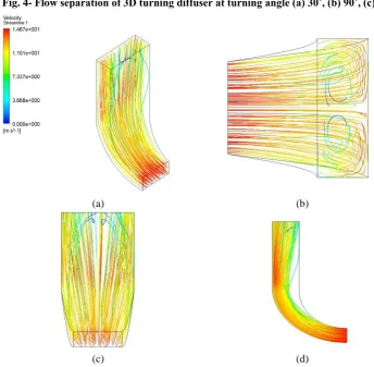
As the turning angle increased from 30˚ to 180˚, the pressure recovery was reduced by 89.3% and the flow uniformity index was raised by 27.7%. Increasing turning angle could further aggravate the presence of reverse flow boundary layer. Therefore, the pressure recovery decreased when turning angle increased. Table 4 shows the tabulated results of pressure recovery, flow uniformity and separation point for 3D turning diffuser with 5 varied angle. Fig. 3 - 5 show how severe the flow is deflected towards the concave region as the angle increased due to flow separation that occurred earliest at S
= 0.44 𝐿𝑖𝑛⁄𝑊1 in particular for 180˚ turning diffuser.
Table 4- Effect of angle of turn on performance of 3D turning diffuser
Angle of turn, ˚ Pressure recovery, 𝑪𝒑 Flow uniformity, 𝝈𝒐𝒖𝒕 Separation point, S
30 0.375 4.548 -
90 0.240 4.733 0.75 𝐿𝑖𝑛⁄𝑊1
120 0.151 4.784 0.63 𝐿𝑖𝑛⁄𝑊1
150 0.103 4.436 0.53 𝐿𝑖𝑛⁄𝑊1
180 0.040 5.808 0.44 𝐿𝑖𝑛⁄𝑊1
Fig. 3-Velocity profile of turning diffuser at varying turning angle 0
2 4 6 8 10 12 14 16 18
0 0.1 0.2 0.3 0.4 0.5 0.6 0.7 0.8 0.9 1
Lo
cal
Ou
tlet Vel
o
city
, V (m
/s
)
Measurement Point Velocity Profile
30 DEGREE 90 DEGREE 120 DEGREE
150 DEGREE 180 DEGREE
No separation
Separation
(a) (b) (c)
Fig. 4- Flow separation of 3D turning diffuser at turning angle (a) 30˚, (b) 90˚, (c) 180˚
(a) (b)
(c) (d)
Fig. 5- Velocity streamline of 90˚ turning diffuser (a) Isometric, (b) Top, (c) Front, (d) Longitudinal views
3.3
Performance Correlations via ACFD
Applying Taylor series expansion on pressure recovery coefficient of 3D turning diffuser, Cp 3DTD acfd:
Cp 3DTD acfd = Cp ref + (ϕ1 – ϕ1 ref)
𝜕𝐶𝑝
𝜕𝜙1 + (ϕ2 – ϕ2 ref) 𝜕𝐶𝑝
𝜕𝜙2 + (ϕ3 – ϕ3 ref) 𝜕𝐶𝑝
𝜕𝜙3 + (ϕ4 – ϕ4 ref) 𝜕𝐶𝑝
𝜕𝜙4 + (ϕ5 – ϕ5 ref) 𝜕𝐶𝑝
𝜕𝜙5 (10)
Rein ref = 6.382 x 10⁴, W2/W1 ref =1.44, X2/X1 ref = 1.50, Lin/W1 ref=4.37, ref = 90o
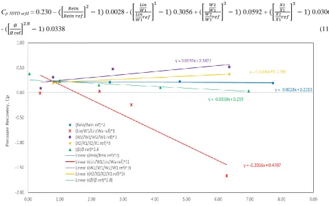
a=2, b=1, c=3, d=3, e=2.8 were selected so that all lines could be fitted in a graph as demonstrated in Fig. 6 and converge at point where Cp ref=0.230.
ϕ1 ref =[
𝑅𝑒𝑖𝑛 𝑅𝑒𝑖𝑛 𝑟𝑒𝑓]
𝑎
= 1.0, thus ϕ2 ref = ϕ3 ref = ϕ4 ref = ϕ5 ref = 1.0
∂Cp
∂ϕ1 = -0.0028, ∂Cp
∂ϕ2 = -0.3056, 𝜕Cp
𝜕ϕ3 = 0.0592, 𝜕Cp
𝜕ϕ4 = 0.0306, 𝜕Cp
𝜕ϕ5 = -0.0338 represented the slopes of the corresponding
lines.
Substituting all the constants in Equation 10 giving,
ϕ1 = [
𝑅𝑒𝑖𝑛 𝑅𝑒𝑖𝑛 𝑟𝑒𝑓]
𝑎
ϕ2 = [
𝐿𝑖𝑛 𝑊1 𝐿𝑖𝑛 𝑊1𝑟𝑒𝑓
] 𝑏
ϕ3 = [
𝑊2 𝑊1 𝑊2 𝑊1𝑟𝑒𝑓
] 𝑐
ϕ4 = [
𝑋2 𝑋1 𝑋2 𝑋1𝑟𝑒𝑓
] 𝑑
ϕ5 = [
Ø Ø 𝑟𝑒𝑓]
Cp 3DTD acfd = 0.230 – ([
𝑅𝑒𝑖𝑛
𝑅𝑒𝑖𝑛 𝑟𝑒𝑓] 2
− 1) 0.0028 - ([
𝐿𝑖𝑛 𝑊1 𝐿𝑖𝑛 𝑊1𝑟𝑒𝑓 ] 1
− 1) 0.3056 + ([
𝑊2 𝑊1 𝑊2 𝑊1𝑟𝑒𝑓 ] 3
− 1) 0.0592 + ([
𝑋2 𝑋1 𝑋2 𝑋1𝑟𝑒𝑓 ] 3
− 1) 0.0306
- ([ Ø Ø ref]
2.8
− 1) 0.0338 (11)
Fig. 6-Outlet pressure recovery, Cp of 3D turning diffuser with respect to ϕ1 =[𝑹𝒆𝒊𝒏⁄𝑹𝒆𝒊𝒏 𝒓𝒆𝒇]𝟐, ϕ2
=[𝑳𝒊𝒏⁄𝑾𝟏⁄𝑳𝒊𝒏⁄𝑾𝟏 𝒓𝒆𝒇]𝟏, ϕ
3 =[𝑾𝟐⁄𝑾𝟏⁄𝑾𝟐⁄𝑾𝟏 𝒓𝒆𝒇]𝟑, ϕ4 = [𝑿𝟐⁄𝑿𝟏⁄𝑿𝟐⁄𝑿𝟏 𝒓𝒆𝒇]𝟑 and ϕ5 = [Ø Ø𝒓𝒆𝒇]⁄ 𝟐.𝟖
Applying Taylor series expansion on pressure recovery coefficient of 3D turning diffuser, 𝜎𝑜𝑢𝑡 3𝐷𝑇𝐷 𝑎𝑐𝑓𝑑:
𝜎𝑜𝑢𝑡 3DTD acfd = 𝜎𝑜𝑢𝑡 ref + (ϕ1 – ϕ1 ref)
𝜕𝜎𝑜𝑢𝑡
𝜕ϕ1 + (ϕ2 – ϕ2 ref) 𝜕𝜎𝑜𝑢𝑡
𝜕ϕ2 + (ϕ3 – ϕ3 ref) 𝜕𝜎𝑜𝑢𝑡
𝜕ϕ3 + (ϕ4 – ϕ4 ref) 𝜕𝜎𝑜𝑢𝑡
𝜕ϕ4
+ (ϕ5 – ϕ5 ref)
𝜕𝜎𝑜𝑢𝑡
𝜕ϕ5 (12)
Rein ref = 6.382 x 10⁴, W2/W1 ref =1.44, X2/X1 ref = 1.50, Lin/W1 ref=4.37, ref = 90o
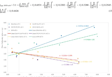
a=2, b=1, c=3, d=3, e=3 were selected so that all lines could be fitted in a graph as demonstrated in Fig. 7 and converge at point where 𝜎𝑜𝑢𝑡 ref=3.1.
ϕ1 ref =[
𝑅𝑒𝑖𝑛 𝑅𝑒𝑖𝑛 𝑟𝑒𝑓]
𝑎
= 1.0, thus ϕ2 ref = ϕ3 ref = ϕ4 ref = ϕ5 ref = 1.0
𝜕Cp
𝜕ϕ1 = 0.6531, 𝜕Cp
𝜕ϕ2 =-0.2202, 𝜕Cp
𝜕ϕ3 = -0.3288, 𝜕Cp
𝜕ϕ4 = -0.2545, 𝜕Cp
𝜕ϕ5 = 0.4426 represented the slopes of the corresponding lines.
Substituting all the constants in Equation 12 giving, ϕ1 = [
𝑅𝑒𝑖𝑛 𝑅𝑒𝑖𝑛 𝑟𝑒𝑓]
𝑎
ϕ2 = [
𝐿𝑖𝑛 𝑊1 𝐿𝑖𝑛 𝑊1𝑟𝑒𝑓 ] 𝑏
ϕ3 = [
𝑊2 𝑊1 𝑊2 𝑊1𝑟𝑒𝑓 ] 𝑐
ϕ4 = [
𝑋2 𝑋1 𝑋2 𝑋1𝑟𝑒𝑓 ] 𝑑
ϕ5 = [
Ø
𝜎𝑜𝑢𝑡 3DTD acfd = 3.1 + ([
𝑅𝑒𝑖𝑛
𝑅𝑒𝑖𝑛 𝑟𝑒𝑓] 2
− 1) 0.6531 - ([
𝐿𝑖𝑛 𝑊1 𝐿𝑖𝑛 𝑊1𝑟𝑒𝑓
] 1
− 1) 0.2202 - ([
𝑊2 𝑊1 𝑊2 𝑊1𝑟𝑒𝑓
] 3
− 1) 0.3288 - [
𝑋2 𝑋1 𝑋2 𝑋1𝑟𝑒𝑓
] 3
− 1) 0.2545 +
([ Ø Ø ref]
3
− 1) 0.4426 (13)
Fig. 7-Flow uniformity index, 𝝈𝒐𝒖𝒕 of 3D turning diffuser with respect to ϕ1 =[𝑹𝒆𝒊𝒏⁄𝑹𝒆𝒊𝒏 𝒓𝒆𝒇]𝟐, ϕ2
=[𝑳𝒊𝒏⁄𝑾𝟏⁄𝑳𝒊𝒏⁄𝑾𝟏 𝒓𝒆𝒇]𝟏, ϕ3 =[𝑾𝟐⁄𝑾𝟏⁄𝑾𝟐⁄𝑾𝟏 𝒓𝒆𝒇]𝟑, ϕ4 = [𝑿𝟐⁄𝑿𝟏⁄𝑿𝟐⁄𝑿𝟏 𝒓𝒆𝒇]𝟑 and ϕ5 = [Ø Ø⁄ 𝒓𝒆𝒇]𝟑
Table 5- Deviations of performance correlations
Correlations Cp 3DTD acfd 𝝈𝒐𝒖𝒕 3DTD acfd
Deviation to CFD (%) 13.7 15.4
Deviation to experiment (%) 7.2 9.4
The ACFD meets adequately both the CFD and experimental results within tolerable deviation as presented in Table 5. Therefore, the developed correlations are dependable to be used to estimate the performance 3-D turning diffuser in future.
4.
Conclusion
The performance correlations of 3D turning diffuser as a function of geometrical and operating parameters was successfully developed using ACFD method. The ACFD results were kept within ±11.4% of deviation when compared with both CFD and experimental results. Therefore, the performance correlations are dependable to evaluate the performance of 3-D turning diffusers.
Acknowledgement
References
[1] Nordin, N., Karim, A. A. Z., Othman, S., Raghavan, V. R., Seri, M. S., & Adzila, S. (2016). Validation by PIV of the numerical study of flow in the 2-D turning diffuser. ARPN Journal of Engineering and Applied Science, 11(20), 11948–11953.
[2] Gan, G., & Riffat, S. B. (1996). Measurement and computational fluid dynamics prediction pressure-loss coefficient. Applied Energy, 54(2), 181-195.
[3] Zainal, B. S. F., Hariri, A., Ismail, M., Abdullah, S., & Kassim, N. I. (2018). Evaluation of respiratory symptoms, spirometric lung patterns and metal fume concentrations among welders in indoor air-conditioned building at Malaysia. International Journal of Integrated Engineering: Special Issue 2018: Mechanical Engineering, 10(5), 109-121.
[4] Balaji, C., Hlling, M., & Herwig, H. (2007). Determination of temperature wall functions for high Rayleigh number flows using asymptotics: A systematic approach. International Journal of Heat and Mass Transfer, 50(19–20), 3820– 3831.
[5] Khong, Y. T., Nordin, N., Seri, S. M., Mohammed, A. N., Sapit, A., Taib, I., Abdullah, K., Sadikin, A. & Razali M. A. (2017). Effect of turning angle on performance of 2-D turning diffuser via Asymptotic Computational Fluid Dynamics. IOP Conference Series: Materials Science and Engineering, 243, 012013.
[6] Seth, N. H., Nordin, N., Othman, S., & Raghavan, V. R. (2013). Investigation of Flow Uniformity and Pressure Recovery in a Turning Diffuser by Means of Baffles. Applied Mechanics and Materials, 465–466, 526–530. [7] Seth, N. H., Mat Isa, N., Othman, S., & Raghavan, V. R. (2016). The effects of angle of attack on 3-dimensional
turning diffuser on baffle performances. ARPN Journal of Engineering and Applied Sciences, 11(3), 1536–1541. [8] Cengel, Y. A., & Cimbala, J. M. (2013). Fluid Mechanics Fundamentals and Applications (3rd ed.) New York:
McGraw-Hill.
[9] Zhang, W., Zhang, Z., Chen, Z., & Tang, Q. (2017). Main characteristics of suction control of flow separation of an airfoil at low Reynolds numbers. European Journal of Mechanics - B/Fluids, 65, 88–97.
[10]Sullerey, R. K., Chandra, B., & Muralidhar, V. (1983). Performance comparison of straight and curved diffusers. Defence Science Journal, 33(3), 195–203.
[11]Nguyen, C. K., Ngo, T. D., Mendis, P. A., & Cheung, J. C. (2006). A flow analysis for a turning rapid diffuser using CFD. Computational Wind Engineering.
[12]Sadikin A., Mohd Y. N. A., Abd H. S. A., Ismail A. E., Salleh S., Ahmad S., Abdol R. M. N., Mahzan S., Ayop S. S (2018). A comparative study of turbulence models on aerodynamics characteristics of a NACA0012 Airfoil. International Journal of Integrated Engineering, 10(1), 134-137.