DOI: https://doi.org/10.30880/ijie.2018.10.04.006
Effect of Path Loss Propagation Model on the Position
Estimation
Accuracy
of
a
3-Dimensional
Minimum
Configuration Multilateration System
Abdulmalik Shehu Yaro
1,2,*, Ahmad Zuri Sha’ameri
11
Department of Electronic and Computer Engineering, School of Electrical Engineering, Universiti Teknologi Malaysia (UTM), Malaysia.
2Department of Communications Engineering, Faculty of Engineering, Ahmadu Bello University (ABU), Zaria,
Nigeria.
Received 10 December 2017; accepted 23 July 2018, available online 5 August 2018
1. Introduction
Passive multilateration system is a wireless position system used by the air navigation service provider (ANSP) to determine the positions of aircraft. The system estimate aircraft position using a two-stage process [1, 2]. The first stage involves estimation of time difference of arrival (TDOA) of the aircraft electromagnetic (EM) emission detected at pairs of ground receiving station (GRS)s [3]. The coordinates of the deployed GRSs are used together with the estimated TDOAs from the first stage as inputs to a lateration algorithm to estimation the aircraft position in the second stage [3]. Several type of approaches to the lateration algorithm have been reported but in this paper, the closed-form lateration algorithm is used [1, 4, 5]. It is the most suitable for passive surveillance purposes and does not surfer convergence issues which is one of the limitations of the other approaches. A 3-dimensional (3-D) or 2-dimensional (2-D) positioning of an aircraft with the MLAT system depends on the number of GRSs deployed. To estimate aircraft position in 3-D, a minimum of four GRSs is used [1].
Several approaches to TDOA estimations have been reported in literatures [6–9] but the most commonly used approach is the cross-correlation (CC) method [8, 9]. The CC method is used particularly in the case of constant delay, stationary process and long observation intervals [9]. In practical applications, signals are corrupted with
noise will leads to TDOA estimation error. Error in the TDOA measurements subsequently results in inaccurate aircraft position estimation (PE) by the MLAT system [2]. The signal-to-noise ratio (SNR) provides a measurement to compare the signal power with respect to the noise power and its value at the any of GRSs varies with different path loss propagation models. Thus, the path loss propagation model between the aircraft and the GRSs contributes to the PE accuracy of the MLAT system [10, 11]. In this paper, the effect of the propagation model on the 3-D PE of a minimum configuration MLAT system is determined. Two models are considered namely Okumura-Hata model and free space path loss (FSPL) model.
The reminder of the paper is organized as follows: Section 2 provide the TDOA estimation methodology based on CC while Section 3 discusses on the signal propagation path loss model and effective SNR. The MLAT PE methodology using the closed-form lateration algorithm is presented in Section 4 followed by the simulation result and discussion in Section 5. Finally, the conclusion is presented in Section 6.
2. TDOA Estimation Methodology
The MLAT system utilizes TDOA measurements that are estimated from the signals received at GRS pairs to perform PE. At each GRS, the received signal is down-converted from radio frequency (RF) to the intermediate Abstract: The 3-Dimensional (3-D) position estimation (PE) accuracy of a multilateration (MLAT) system depends on several factors one of which is the accuracy at which the time difference of arrival (TDOA) measurements are obtained. In this paper, signal attenuation is considered to be the major contributor to the TDOA estimation error and its effect based on path loss propagation model on the PE accuracy of the MLAT system is determined. The two path loss propagation models considered are: Okumura-Hata and the free space path loss (FSPL) model. The transmitter and receiver parameters used for the analysis are based on actual system used in the civil aviation surveillance. Monte Carlo simulation result based on square ground receiving station (GRS) configuration and at some randomly selected aircraft positions show that the MLAT system with the Okumura-Hata model has the highest PE error. The horizontal coordinate and altitude errors obtained considering the Okumura-Hata are 2.5 km and 0.6 km respectively higher than that obtained with the FSPL model.
frequency (IF), which is then used for the TDOA estimation process. The transmitted signal is defined as:
( )
( ) cos(2
c)
( )
x t
m t
f t rect t
(1)
where 𝑚(𝑡) is the message content of the signal, 𝑓𝑐 is the carrier frequency of the signal, and 𝑟𝑒𝑐𝑡(𝑡) is a rectangular function defined as:
1
0
( )
0
elsewhere
t
T
rect t
(2)The signal received at the i-th and the m-th GRSs respectively are:
( )
(
)
( )
i i i
x t
x t
n t
(3)( )
(
)
( )
m m m
x t
x t
n t
(4)where 𝜏𝑖 and 𝜏𝑚 are the delays in the signal received by the i-th and the m-th GRSs respectively. 𝑛𝑖(𝑡) and 𝑛𝑚(𝑡)
that are independent uncorrelated noise sources with zero mean and variance 𝜎𝑛,𝑖2 and 𝜎𝑛,𝑗2 respectively.
The CC is used to estimate the TDOA between the received signal obtained at GRS pair and is defined as [9]:
( )
[ ( )
(
)]
i m
x x i m
R
E x t x t
(5)
The TDOA (𝜏𝑖𝑚) between the signals estimated from the peak of CC from Eq. (5) is:
arg_max
( )
i m
im
R
x x
(6)
TDOA estimation error is produced due to the noise present in the signal, as shown in Eq. (6). Modelling the error as zero mean Gaussian random variable with normal probability density function, the estimated TDOA measurement is [12]:
ˆ
im imN
0,
im
(7)where
im is the TDOA estimation error standard deviation (SD) and in this paper, it is assumed to depends on the effective SNR between the i-th and m-th GRS pair.
3.
Signal Propagation Model and Effective
SNR
In Section 2, it was concluded that the TDOA estimation error SD depends on the effective SNR between GRSs. The SNR of the signal at each GRS
propagation model. Table 1 shows a comparison in terms base station (BS) antenna height, mobile station (MS) antenna height, frequency operation ranges and maximum valid coverage of three commonly used outdoor path loss models.
Table 1: Outdoor propagation model parameter comparison [13, 14].
Parameter
Path loss model
Okumura-Hata model
Hata
model COST 231
MS antenna
Height (m)
1 to 3 1 to 10 1 to 10
BS antenna
Height (m)
30 to 1000 30 to 200 30 to 200
Frequency Range (MHz)
150 to 1920 150 to 1500 1500 to 2000
Coverage
(km) ≤ 100 ≤ 10 ≤ 20
In the context of MLAT system, the BS antenna height corresponds to the altitude of the aircraft from the horizontal plane while the MS antenna height corresponds to GRS antenna height. According to international civil aviation organisation (ICAO) standard, the minimum safe altitude (MSA) at which an aircraft can fly is 1000 ft (~300 m) [15]. This means that the Hata and COST 231 propagation model cannot be used in calculating the SNR of the signal at each GRS as the maximum antenna height to enable the used of these models is 200 m. Thus, in this paper, the signal propagation path loss model considered for estimation of received SNR at each GRS are the Okumura-Hata and free space path loss (FSPL) model.
3.1
Path Loss Model
In this section of the paper, mathematical derivations of the signal attenuation based on the FSPL and Okumura-Hata propagation model is presented.
3.1.1
Signal Attenuation based on FSPL
Propagation Model
The FSPL model is used under the assumption that the aircraft and GRS have a clear and unobstructed line-of-sight (LOS) path between them. For an aircraft located at coordinates (𝑥, 𝑦, 𝑧), the FSPL attenuation of the signal received at the i-th GRS with coordinate (𝑥𝑖, 𝑦𝑖, 𝑧𝑖) is
mathematically expressed as [14]:
,
32.44 20 log (
10)
20 log (
)
FPSL i i
PL
dB
d
f
where 𝑓𝑐 is the carrier frequency of the signal in MHz and
𝑑𝑖 is the 3-D Euclidean distance between the aircraft and
the i-th GRS obtain using Eq. (9).
2
2
2i i i i
d
x
x
y
y
z
z
(9)3.1.2
Signal attenuation based on
Okumura-Hata Path Loss Propagation Mode
In the calculation of the signal attenuation, Okumura-Hata model takes into account several propagation parameters such as the terrain irregularity, building type and density. Mathematically, the signal attenuation at the
i-th GRS for a medium-small city based on Okumura-Hata model is [13]:
, 10 10 10(
)
69.55 26.16 log
13.82 log
44.9 6.55log
okumura i c
i i
PL
dB
f
z
a z
d
(10) where
10 101.1log
0.7
1.56 log
0.8
c i
c
K
f
z
f
(11)
3.2
Effective SNR between GRS pair
The received power at the i-th GRS is mathematically obtained as:
i
r t t r i
P
P
G
G
PL
(12)where 𝐺𝑡 and 𝐺𝑟 respectively are the transmit and
received antenna gain in dBi and 𝑃𝐿𝑖 is the signal
attenuation obtained using either Eq. (8) or Eq. (10). The received SNR at the i-th GRS is now obtained as:
i i r n
SNR
P
P
(13)where 𝑃𝑛 is the receiver sensitivity in dBm.
TDOA estimation involves the use of GRS pairs. Let the m-th GRS be the GRS paired with the i-th GRS (as reference) for the TDOA estimation. The received SNR at the m-th GRS based on Eq. (13) is
m
m r n
SNR
P
P
(14)The effective SNR for the TDOA estimation between the
i-th and m-th GRS pair is mathematically obtained as [16]:
,
1
1
1
1
min
,
i m eff
i m i m
i m
SNR
dB
SNR
SNR
SNR
SNR
SNR SNR
(15)4.
MLAT Position Estimation Methodology
After the TDOA measurements have been estimated from GRS pairs, the next stage is the estimation of the location of the aircraft using the lateration algorithm. The TDOA measurement in Eq. (7) is related to the aircraft position as follows:
2 2 2
2 2 2
ˆ
ˆ
im im
i i i
m m m
d
c
x
x
y
y
z
z
x
x
y
y
z
z
(15)
Eq. (15) is known as the range difference (RD) equation which corresponds to the distance equivalent of the TDOA measurements in Eq. (7). Also, the RD estimation (RDE) error SD is the distance equivalent of the TDOA estimation error SD. With a total of four GRSs and GRS pair as reference, four independent RD equations in the form of Eq. (15) are obtained [1]. Let the remaining two GRSs be labelled j-th and k-th. With the i-th and j-th GRS as reference stations for TDOA estimation and the m-th and k-th as non-reference stations, the remainder of the three RD equation are
2 2 2
2 2 2
ˆ
ik i i i
k k k
d
x
x
y
y
z
z
x
x
y
y
z
z
(16)
2 2 2
2 2 2
ˆ
jm j j j
m m m
d
x
x
y
y
z
z
x
x
y
y
z
z
(17)
2 2 2
2 2 2
ˆ
jk j j j
k k k
d
x
x
y
y
z
z
x
x
y
y
z
z
(18)
Algebraic manipulation of Eq. (15) to Eq. (18) as done in [1], two 3-D plane equations are obtained as follows:
, , , , , , , , i k m i k m i k m i k m
A
xB
yC
zD
(19), , , , , , , ,
j k m j k m j k m j k m
where the coefficients of Eq. (19) and Eq. (20) depends on RD measurements and GRSs coordinates which can be found in [1].
The unknown in Eq. (19) and Eq. (20) is the aircraft position (𝑥, 𝑦, 𝑧). To solve for the aircraft position, the horizontal coordinates x and y are expressed as a function of altitude z resulting into two equations [1]. The two equations which are function of z are substituted into one of the RD equations i.e. Eq. (15) and further simplification will result in a second order quadratic equation as a function of z. The solution to the second order quadratic equation with the positive value is chosen as the estimate aircraft altitude which is then substituted into the earlier obtained equations for the 𝑥 and 𝑦 to obtain the estimated horizontal coordinates. Detail derivations of the procedure to obtain the aircraft position using Eq. (19) and Eq. (20) is presented in [1].
Aircraft positions for surveillance purposes are displayed in terms of range (𝑅), bearing (𝜃) and altitude
𝑧 which corresponds to the cylindrical coordinate system. In the remainder of the paper, aircraft positions will be defined in cylindrical coordinate system that is
(𝑅, 𝜃, 𝑧) and conversion from the cylindrical coordinate to Cartesian coordinate system can be done using Eq. (21).
cos
x
R
(21a)
sin
y
R
(21b)z
z
(21c)4.1.Reference Station Selection for TDOA
Estimation
Beside TDOA measurement error, another factor that contribute to the PE accuracy of the MLAT system is the choice of reference station for TDOA estimation. In this paper, reference station selection technique proposed in [1] is adopted. A matrix 𝐌𝑖𝑗 was derived that has as its entries only the RD measurements as shown in Eq. (22).
1
0
ˆ
ˆ
1
0
ˆ
ˆ
im in ij jm jnd
d
d
d
M
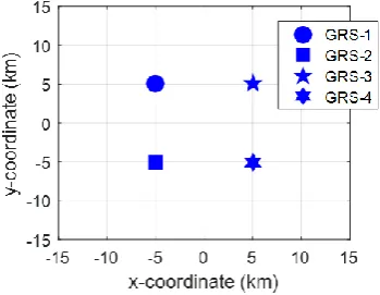
(22)With four GRSs and GRS pair as reference, six possible combinations of reference station pair are obtained. Let the deployed GRSs be GRS-1, GRS-2, GRS-3 and GRS-4, summary of all the possible reference station pair combinations is presented in Table 2. Each of the reference station pair combinations in Table 2 is used in generating RD measurements which are substituted into the matrix in Eq. (22). The reference station pair
combination whose PD measurements resulted in the least condition number value is chosen to be used with the lateration algorithm for PE.
Table 2: Possible combinations of reference stations pairs
GRS pair
Reference stations
Non-reference station
i-th j-th m-th n-th Pair 1 GRS-1 GRS-2 GRS-3 GRS-4 Pair 2 GRS-1 GRS-3 GRS-2 GRS-4 Pair 3 GRS-1 GRS-4 GRS-2 GRS-3 Pair 4 GRS-2 GRS-3 GRS-1 GRS-4 Pair 5 GRS-2 GRS-4 GRS-1 GRS-3 Pair 6 GRS-3 GRS-4 GRS-1 GRS-2
5.
Results and Discussion
In this section of the paper, the effect of the path loss propagation models presented in Section 3 on the PE accuracy of the MLAT system is presented. The position root mean square error (RMSE) is used as the performance measure to evaluate the PE accuracy of the MLAT system. Mathematically, the horizontal coordinate and altitude RMSE is mathematically expressed as:
2 2 1 ˆˆ cos( ) cos( ) 1
ˆ
ˆ sin( ) sin( )
N n n
rmse
n
n n
R R
H
N R R
(23a)
21
1
ˆ
N rmse n nZ
z
z
N
(23b)where (𝑅, 𝜃, 𝑧) is the known aircraft position and
(𝑅̂𝑖, 𝜃̂𝑖, 𝑧̂𝑖) is the estimated aircraft position at the n-th
Monte Carlo simulation realization (𝑁 = 100).
For the analysis, the squared GRS configuration is considered which has been shown in [1, 17] to produce the best PE performance. The distribution of the GRS is shown in Fig. 1.
Fig. 1: Square GRS configuration with 5 km separation
Table 3: Transmitter and receiver simulation parameters
Parameter Value
Transmit power 250 Watt
Carrier frequency 1090 MHz
GRS receiver sensitivity -90 dBm GRS antenna gain 12 dBi
Transmitter antenna gain 3 dBi
(a) Okumura-Hata path loss model
(b) FSPL
Fig. 2: Effective SNR comparison within 100 km MLAT coverage radius
5.1
Effective SNR and RDE Error SD
Comparison
In this section of the paper, the effective SNR between GRS pair obtain using the FSPL model based on Eq. (8) and the Okumura-Hata path loss model based on Eq. (10) are obtained and compare for aircraft positions within 100 km coverage radius and at 1 km altitude. Fig.
2 shows the effective SNR comparison between the two path loss models. Irrespective of the path loss model used, the effective SNR increases with increase in the aircraft horizontal range from 0 km to 100 km but remains constant with change in the aircraft bearing. Comparison between the two-path loss model shows that the Okumura-Hata model has the least effective SNR. For instance, at an aircraft horizontal range, 𝑅 = 50 𝑘𝑚, the effective SNR based on the Okumura-Hata model is 17 dB while based on the FSPL model is 31 dB. On the average, within the 100-km coverage radius, the Okumura-Hata path loss model results in an SNR that is 14 dB less than the FSPL model.
(a) Okumura-Hata path loss model
(b) FSPL
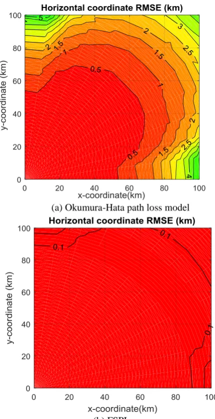
(a) Okumura-Hata path loss model
(b) FSPL
Fig. 4: Horizontal coordinate RSME comparison
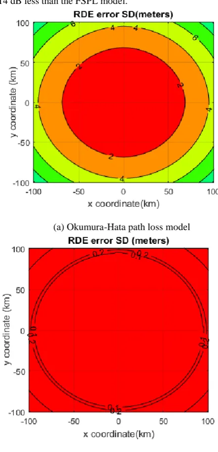
Using the effective SNR at each aircraft position, the RDE error SD for the two path loss models are obtained and compare as shown in Fig. 3. Irrespective of the path loss model, the RDE error SD varies with aircraft position. It increases with increase in range from 0 km to 100 km but relatively constant with change in bearing. RDE error comparison for the two-path loss model shows higher RDE error SD with the Okumura-Hata path loss model as compared to the FSPL. This is due to low values of effective SNR obtained using the Okumura-Hata path loss model.
The RDE error SD at each aircraft position is used in obtaining the estimated RD equations which are subsequently used in generating the two plane equations in Eq. (19) and Eq. (20). These equations are used to obtain the estimated aircraft positions. The accuracies at which aircraft positions are estimated for both the Okumura-Hata and FSPL model are determined and compared in the next section.
5.2
MLAT PE Accuracy Comparison
In this section of the paper, the PE accuracies comparison of the MLAT system based on the Okumura-Hata and FSLP model are obtained and compared. From section 5.1, it is seen that the RDE error SD dependent only on the aircraft range. Thus, for this reason, PE accuracy of the aircraft is determined for bearing range of 00 to 900.
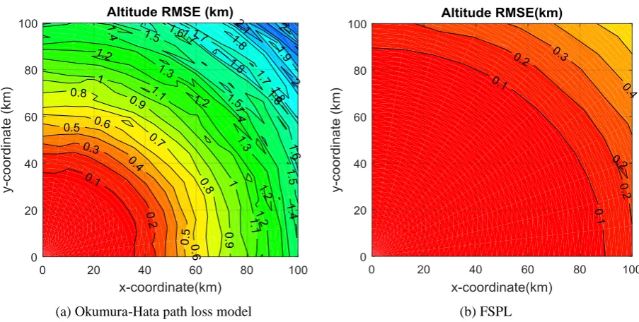
Fig. 4 and Fig. 5 shows the horizontal coordinate and altitude RMSE comparison based on Eq. (23) of the MLAT system using the Okumura-Hata and FSPL model. The position RMSE increases with increase in the aircraft range from 0 km to 100 km. It remains relatively constant with the change in aircraft bearing. Table 4 show the position RMSE error comparison obtained by the two path loss models at some selected aircraft positions. The position RMSE obtained with the Okumura-Hata model is higher than that obtained with the FPSL model at all aircraft positions considered. For instance, at aircraft position E, the horizontal coordinate and altitude RMSEs of the MLAT system with the Okumura-Hata path loss model are 200 m and 420 m while for the with the FSPL model the position RMSE is 0 m. The high position RMSE obtained with the Okumura-Hata path loss model is due to the low effective SNR between GRS pairs. This is because other propagation parameters such as the terrain irregularity are considered in the signal attenuation calculation unlike the FSPL model which assume clear unobstructed path between the aircraft and the GRSs. On the average, based on the selected aircraft positions, the horizontal coordinate and altitude RMSE of the MLAT system based on the Okumura-Hata model path loss model are 2500 m and 600 m respectively higher than that obtained using the FSPL model.
6.
Summary
References
[1] Yaro, A.S., Sha’ameri, A.Z., and Kamel, N. Ground Receiving station reference pair selection technique for a minimum configuration 3-D emitter position estimation multilateration system. Advances in Electrical and Electronic Engineering, Volume 15, (2017), pp. 391–399.
[2] Mantilla-Gaviria, I.A., Leonardi, M., Galati, G., and Balbastre-Tejedor, J. V. Localization algorithms for multilateration (MLAT) systems in airport surface surveillance signal. Image and Video Processing, Volume 9, (2015), pp. 1549–1558.
[3] Zekavat, R., and M. Buehrer, R. Handbook of position location: Theory, practice and advances. John Wiley & Sons, Inc. (2012).
[4] Stojilovi, M., Menssen, B., Flintoft, I., Garbe, H., Dawson, J., and Rubinstein, M. TDoA-based
localisation of radiated IEMI sources.
Proceeding of IEEE International Symposium on Electromagnetic Compatibility, (2014), pp. 1263–1268.
[5] Weng, Y., Xiao, W., and Xie, L. Total least squares method for robust source localization in sensor networks using TDOA measurements. International Journal of Distributed Sensor Networks, Volume 7, (2011), pp. 172902.
[6] M. Shamian, Z., Hadi, A., and Ijaz, K. Ultra-wide band localization and tracking hybrid technique using VRTs. International Journal of Integrated Engineering, Volume 4, (2012), pp. 65–71.
[7] Dou, H., Lei, Q., Li, W., and Xing, Q. A new TDOA estimation method in three-satellite interference localization. International Journal of Electronics, Volume 102, (2015), pp. 839–854.
(a) Okumura-Hata path loss model (b) FSPL
Fig. 5: Altitude RSME comparison
Table 4: Position RMSE comparison. Green shade indicates path loss model with the least position RMSE.
Aircraft position
Position RSME (m)
Horizontal coordinate RMSE Altitude RMSE Range
(km)
Bearing (0)
Altitude
(km) Okumura-Hata FSPL Okumura-Hata FSPL Aircraft A 10
10
1
0 0 0 0
Aircraft B 20 0 0 0 0
Aircraft C 30
20 50 0 50 0
Aircraft D 40 150 0 150 0
Aircraft E 50
40 200 0 420 0
Aircraft B 60 450 0 700 0
Aircraft F 70
60 1000 0 1000 0
Aircraft G 80 1730 0 1300 0
Aircraft H 90
80 8860 0 1460 0
[8] Marmaroli, P., Falourd, X., and Lissek, H. A comparative study of time delay estimation techniques for road vehicle tracking. Proceeding of 11th French Congress of Acoustics and 2012 Annual IOA Meeting, (2012), pp. 136–140.
[9] Shi, H., Zhang, H., and Wang, X. A TDOA technique with super-resolution based on the volume cross-correlation function. IEEE Transactions on Signal Processing, Volume 64, (2016), pp. 5682–5695.
[10] Hu, Y., Zhang, L., Gao, L., Ma, X., and Ding, E. Linear system construction of multilateration based on error propagation estimation. EURASIP Journal on Wireless Communications and Networking, Volume 2016, (2016), pp. 154–164.
[11] Abdulqader, H., Rahman, T. A., and Leow, C. Performance evaluation of localization accuracy for a log-normal shadow fading wireless sensor network under physical barrier attacks. Sensors, Volume 15, (2015), pp. 30545–30570.
[12] Galati, G., Leonardi, M., Balbastre-Tejedor, J.V., and Mantilla-Gaviria, I.I.A. Time-difference-of-arrival regularised location estimator for multilateration systems. IET Radar, Sonar & Navigation, Volume 8, (2014), pp. 479–489. [13] Beire, A.R., Cota, N., Pita, H., and Rodrigues, A.
Automatic tuning of Okumura-Hata model on railway communications. Proceeding of IEEE Symposium on Wireless Personal Multimedia Communications, (2014), pp. 562–567.
[14] Artemenko, O., Rubina, A., Harishchandra Nayak, A., Baptist Menezes, S., and Mitschele-Thiel, A. Evaluation of different signal propagation models for a mixed indoor-outdoor scenario using empirical data. Transactions on Mobile Communications and Applications, Volume 2, (2016), pp. 151–159. [15] Mark, J.C. and Jason, Z. Navigable Airspace:
Where Private Property Rights End and Navigable Airspace Begins. Fox Rothschild, (2016). Available online:
https://ontheradar.foxrothschild.com/2016/01/article s/general-uas-news-and-developments/navigable- airspace-where-private-property-rights-end-and-navigable-airspace-begins/
[16] Yaro, A.S., Sha’ameri, A.Z., Kamel, N. Position estimation error performance model for a minimum configuration 3-D multilateration. International Journal on Electrical Engineering and Informatics, Volume 10, (2018), pp. 153–169.
[17] Bais, A., Kiwan, H., and Morgan, Y. On optimal placement of short range base stations for indoor position estimation. Journal of Applied Research and Technology, Volume 12, (2014), pp. 886–897. [18] SELEX Sistemi Integrati: ‘ADS-B Subsystem:
Standard E5010015201SDD’ (2014)
[19] Francis, R., Vincent, R., and Noël, J.M. The flying laboratory for the observation of ADS-B signals.
International Journal of Navigation and Observation, Volume 2011, (2011), pp. 1–5.
![Table 1: Outdoor propagation model parameter comparison [13, 14]. Path loss model](https://thumb-us.123doks.com/thumbv2/123dok_us/8438437.1700420/2.595.297.545.165.362/table-outdoor-propagation-model-parameter-comparison-path-model.webp)