R E S E A R C H
Open Access
Towards negative cycle canceling in wind
farm cable layout optimization
Sascha Gritzbach
*, Torsten Ueckerdt, Dorothea Wagner, Franziska Wegner and Matthias Wolf
FromThe 7th DACH+ Conference on Energy Informatics Oldenburg, Germany. 11–12 October 2018
*Correspondence:
Karlsruhe Institute of Technology, Department of Theoretical Informatics, Karlsruhe, Germany
Abstract
In the WINDFARMCABLINGPROBLEM(WCP) the task is to design the internal cabling of a wind farm such that all power from the turbines can be transmitted to the substations and the costs for the cabling are minimized. Cables can be chosen from several available cable types, each of which has a thermal capacity and cost. Until now, solution approaches mainly use MIXED-INTEGERLINEARPROGRAMs (MILP) or metaheuristics. We present our current state of research on a fast heuristic specifically designed for WCP. We introduce an algorithm that iteratively improves a cable layout by finding and canceling negative cycles in a suitably defined network. Our simulations on publicly available benchmark sets show that the heuristic is not only fast but it tends to produce good results. Currently our algorithm gives better solutions on large wind farms compared to an MILP solver. However, on small to medium instances the solver performs better in terms of solution quality, which represents a starting point for future work.
Keywords: Wind farm cable layout, Negative cycle canceling, Network flow, Step function, Heuristic
Introduction
In view of the European Union’s ‘2030 Energy Strategy’, which, among other things, aims at having “at least a 27% share of renewable energy consumption” (European Commission
2018), renewable energy sources have become increasingly important. In terms of elec-tricity, the gross generation in the EU28 in 2016 came with a 30.2% share from renewable energy, out of which a 30.9% share was due to wind energy (European Commission DG ENER Unit A42018). WindEurope states that in 2017, additional 15,638 MW of wind power capacitity were installed in the EU28, out of which 3154 MW come from offshore wind farms (WindEurope asbl/vzw2018).
A typical offshore wind farm consists of turbines and substations. Turbines convert wind energy to electricity which is transported through medium-voltage sea cables, possibly via other turbines, to substations (internal cabling) where the electricity is trans-formed to the high-voltage level and transported to an onshore grid point (external cabling).
In the process of planning wind farms, various stages have to be completed. Turbines have to be placed in a way to maximize wind usage and minimize wake effects, substations should be close to the turbines and both the internal and the external cabling need to be found adhering to geographical, economic, and electrical constraints. Ideally, an optimal planning process would unify all stages in a single process.
With the increasing size of newly planned wind farms (e.g., Hornsea Project Three may include up to 300 turbines (Hornsea Project Three Offshore Wind Farm2018)), planning by hand becomes more difficult and hence automated approaches become more desirable. Automated approaches, however, tend to have difficulties with the complexity of a unified planning process (Santos et al.2014), which leads to considering subsets of the planning stages separately.
The cost for the internal cabling accounts for approximately 17% of the total cost for planning and building a wind farm (Santos et al.2014). Therefore, it is essential to find a cost-efficient cabling. When designing the internal cabling isolatedly, the positions of turbines and substations are considered fixed and grid points and high-voltage cabling are not of interest at this time. Also as an input to the problem, there are given possible connections between turbines and between turbines and substations. These connections can be used for routing the electricity produced by the turbines. Furthermore, there is a set of possible cable types that can be installed on the connections in order to transmit electricity. Each cable type has a thermal capacity and a cost per unit length for mate-rial and installation. The goal of this planning stage is to identify connections on which electricity is routed and to assign a cable type to every connection such that all electricity can be transported to substations. We call this planning stage the WINDFARMCABLING
PROBLEM(WCP). SinceWCPincludes the NP-hard problem CAPACITATED MINIMUM
SPANNINGTREE(Cerveira et al.2014), it is NP-hard as well.
Contribution and Outline We present a basic implementation of a heuristic forWCP, which first computes a feasible solution and iteratively improves it by finding and can-celing negative cycles in a suitably defined graph. To find these negative cycles we use a slight modification of the Bellman-Ford Algorithm (Bellman1958; Ford et al. 2010). Evaluating the heuristic on the wind farm benchmark sets presented by Lehmann et al. (2017) shows that it runs fast and gives good results compared to the solution com-puted by the MILP solver Gurobi (Gurobi optimizer reference manual 2018) within one hour.
In the following section we review the literature on the WINDFARMCABLINGPROB
-LEM (WCP), applications of negative cycle canceling, and other related problems. We modelWCPformally in the “Model” section. In the “Algorithmic overview” section, we explain our heuristic in detail. We report and discuss the results of the simulation of our heuristic in the “Simulations” section and conclude with a thorough overview of possible research directions.
Related work
For finding the optimal cable layout between turbines and substations with fixed positions—which is also the scope of this work—one of the first papers was by Berzan et al. (2016), in which they propose a hierarchical decomposition of the problem into several layers. They use well-studied graph problems to solve the so-called Circuit and Substation layers, in which only one substation is considered at a time, when there is only one cable type available.
Since then, various approaches have been taken for more elaborate problems consider-ing different optimization functions and sets of constraints. With the high complexity of the problem in mind, metaheuristics, such as Genetic Algorithms (Zhao et al.2004; Shir-shak et al.2017; Dahmani et al.2015) or Simulated Annealing, (Lehmann et al.2017) are very popular. While these approaches do not guarantee provably optimal solutions, they are able to provide good solutions within short running times. To the contrary, exact solu-tions can be provided by IN TEGERLINEARPROGRAM(ILP) or MIXED-IN TEGERLINEAR
PROGRAM(MILP) formulations, which need more time and therefore only work on small
instances. Lumbreras and Ramos (2013), for example, consider losses along branches, stochasticity in wind inputs and component failures in an ILP and Cerveira et al. (2014) use a graph-theoretic flow model on wind farms with a single substation and use the resemblance to the CAPACITATED MINIMUMSPANNINGTREE (CMST). Based on the flow model, they include constraints representing the CMST into anMILPformulation.
In our work, we use a flow model similar to the one presented by Cerveira et al. (2014) representing how turbine production is routed to one of multiple substations. We aim at finding a flow of minimum cabling cost and apply a well-known technique from network flow theory callednegative cycle canceling. Negative cycle canceling was first proposed in the context of finding minimum cost circulations in flow networks (Klein1967). Goldberg and Tarjan (1989) achieve a strongly polynomial running time for a cycle-canceling-based algorithm for the minimum cost flow by suitably choosing the cycles to cancel. The bound for the running time of this algorithm was later tightened by Radzik and Goldberg (1994). Ouorou and Mahey (2000) employ negative cycle canceling to solve the Minimum Multicommodity Flow Problem with nonlinear cost functions. Negative cycle cancel-ing is also used in combination with tabu search to tackle the Capacity Expansion Problem for multicommodity flow networks (de Souza et al. 2008), which can be modeled as a Multicommodity Flow Problem with non-convex and non-smooth cost functions.
Optimization problems that are similar toWCPappear for example in logistics. In the Single-Sink Edge Installation Problem introduced by Salman et al. (2001) the production of multiple sources must be transported to a single sink. On every connection a mixture of various cable types (including multiple copies of the same type) needs to be installed such that the cables provide sufficient capacity. Similarly, in the Buy-at-Bulk Problem (see (Gupta and Könemann2011)), the cost of routing flow along a connection is given by a concave function representing economies of scale. In both cases, the amount of flow on a single connection is unlimited.
Our approach, on the other hand, has been tested on instances with up to 500 vertices providing good solutions within 50 seconds on average and 7.5 minutes in the worst case.
Model
In this section, we formalize the WINDFARMCABLINGPROBLEM(WCP). We understand turbines and substations as vertices of a graphG= (V,E), i.e., ifVT andVSdenote the sets of turbines and substations, respectively, thenV = VT ∪VS andVT ∩VS = ∅. While the direction of a connection between a turbine and a substation or between two turbines does not matter in the real world, for the sake of modeling we impose an arbitrary direction on every connection. This implies thatGis a directed graph, i.e., for every edgee
there are verticesuandvsuch thate=(u,v)and we sayegoes fromutov. We assume that turbine production that is transmitted to a substation is transmitted into the connection to the grid point. In particular, it is not routed to a second substation first. To simplify the description of our algorithm, we therefore assume that there are no edges connecting two substations. Moreover, we assume that each turbine has a standardized production of one unit and each substation has a capacity modeled by a function capsub: VS → N. Additionally, each edge is assigned a positive length by the function len :E→R>0, which
represents the geographic distance between the endpoints of the edge.
Along each edge we may place a single cable, whose type is chosen from a finite set of cable types. Each cable type is uniquely determined by its capacity capcab ∈ Nand its cost per unit length ccab ∈ R≥0. We therefore identify each cable type with the pair
(capcab, ccab)and define the setK of all allowed cable types represented by these pairs.
For the ease of representation we assume thatKcontains the two special cable types(0, 0) and(∞,∞)calledtrivial cable types. The former represents the case that no cable is built along an edge and the latter the case that no cable has sufficient capacity. Based on the cable types we define a cost function c :Z→R≥0∪ {∞}by
c(x)=min{ccab:(capcab, ccab)∈K,|x| ≤capcab} ∀x∈Z, (1)
i.e., we choose the cheapest cable type that has sufficient capacity to transport|x|units of flow.
In total, a wind farm is then modeled as a networkN =(G,VT,VS, len, capsub, c). The
network incorporates turbinesVT, substationsVSwith a capacity capsubeach, and
con-nections between turbines and substations described by the graphG, as well as the length of the connections len and costs per length c for using the connections. Note that we do not explicitly include the set of cable typesKas all necessary information on them is incorporated in the function c.
A flow in the network N is a function f: E → R. Since we imposed an arbitrary direction on each edge, we are able to identify the direction of a flow on an edge. More formally, iff(u,v) >0 (resp.<0) for some edge(u,v), we interpret that asf(u,v)(resp. −f(u,v)) units flowing from u to v (resp. from v to u). For every vertex u we define itsnet flowbyfnet(u)=(w,u)∈Ef(w,u)−
fnet(u)= −1 ∀u∈VT, (2)
fnet(u)≤capsub(u) ∀u∈VS, (3)
f(u,v)≥0
f(v,w)≤0 ∀v∈VS, ∀(u,v),(v,w)∈E (4)
Thecostsof a feasible flowf are computed as the sum of the individual costs of every edge.
cost(N,f)=
e∈E
c(f(e))·len(e). (5)
The goal of WCP is to find a feasible flow f with minimum costs. Hence, it can be summarized as follows.
Negative cycle algorithm
In this section, we describe an approach of finding and canceling negative cycles in order to solveWCPheuristically. The main idea of our heuristic is to repeatedly set up a residual graph from a flow, finding a negative cycle, and cancel negative cycles in the residual graph. Every cancellation yields a better solution to WCP. In the first part, we give an overview of our heuristic. Whereas in the second part, we describe the components used in the heuristic in more detail.
Algorithmic overview
Before we describe the algorithm, we introduce essential graph theoretical terms. We define awalkfromutowas a sequence of—not necessarily distinct—edges((u,v1) =:
e0,e1,. . .,ek:=(vk,w))such that the end vertex ofei−1is the same as the start vertex ofei fori∈ {1,. . .,k}. A walk isclosedifu=wand it isside-trip freeifeiis not the reverse edge ofei−1for alli ∈ {1,. . .,k}, i.e., the walk does not contain a closed subwalk of length 2.
Closed walks where the end vertices of all edges are distinct are calledcycles.
Given a wind farmN we first compute an initial feasible flowf (Lines2–4; all line references in this section refer to Algorithm1). For each turbineu ∈ VT we perform a breadth-first search fromu ignoring all edges and substations without free capacity. When the search finds a substation for the first time, the flow on the path fromuto the substation is increased by 1. Starting with this initial flow, we iteratively identify simple changes of the flow that decrease the costs.
Algorithm 1:Our Heuristic forWCP
Input: A wind farmN =(G,VT,VS, len, capsub, c).
Result: A feasible flowf onGwhose costs cannot be improved by canceling negative cycles in any residual graph.
1 f(e):=0 ∀e∈E
2 foru∈VT do
3 π:= BFS(N, u, f ) ignores all edges and substations without free capacity
4 f(e)++ ∀e∈π
5 :=0
6 while <2·max{x∈Z: c(x) <∞}do
7 ++; :=
8 R := getResidualGraph(N, f,)
9 W := NegativeCycleDetection(R) Bellman-Ford Algorithm
10 forcycle C in Wdo
11 ife∈Cγ (e) <0and|C|>2 then
12 f :=NegativeCycleCancellation(C,f,) see Eq.6
13 :=0
14 :=
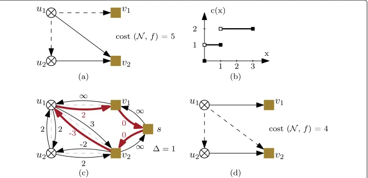
Letf be the flow computed in the previous iteration and ∈ Nwith initialization shown in Lines5and7. In addition, we define the cost functionγ:E(R)→Ras explained below. We then search for a closed side-trip-free walk with negative total costs in R (Line9). To this end, we use a slight adaptation of the Bellman-Ford Algorithm. If there is no such walk, we incrementand set up a new residual graph. Otherwise, if there is such a walkWinR, we splitW into cyclesC1,. . .,Cl. Figure1shows an example of this decomposition into cycles. We check for each cycleCi whether its total costs are nega-tive and whetherCihas length at least 3 (Line11). If both conditions hold, we cancelCi (see Eq.6and Line12). Note that the cost functionγ is defined in such a way that cycles that decrease the cost have negative total costs. Wecancel Cby changing the flowf by alongC. More formally, we define a new flowffor all(u,v)∈E(G)by
f(u,v)=
⎧ ⎪ ⎨ ⎪ ⎩
f(u,v)+, if(u,v)∈E(C),
f(u,v)−, if(v,u)∈E(C),
f(u,v), if(u,v),(v,u)∈E(C).
(6)
Here,E(C)denotes the set of edges that form the cycleC; see Fig.2for an example of canceling a cycle.
Note that if a cycle has length exactly 2, it consists of an edge(u,v)and its reverse(v,u). Hence, canceling it means sendingunits in both directions specified by(u,v)and(v,u), which does not change the flow. Canceling it would result in an infinite loop in Line10.
Finally, if at least one cycleCi inW was canceled, we resetto 1 and build a new residual graph based on the new flow after the cycle cancellation in the current iteration. The heuristic terminates once it does not cancel a negative cycle in the residual graphs of the currently cheapest feasible flow for all values of.
The residual costs
The description above assumes a cost functionγ on the residual graphRsuch that nega-tive cycles inRcorrespond to cycles that decrease the costs of the flow if they are canceled. We defineγ in this section.
Letf be a feasible flow inN and ∈ N. We defineγ: E(R) → R∪ {∞}such that canceling a cycle with negative costs, i.e., a cycle C withe∈E(C)γ (e) < 0, preserves feasibility and reduces the total costs. Consider an edge(u,v)∈E(G). Intuitively,γ (u,v)
represents the change of costs for the original flowf(u,v)if additionalunits are sent fromutov. More formally, if bothuandvare turbines, the costs of the corresponding edges in the residual networkRare defined by
γ (u,v)=
cf(u,v)+−cf(u,v)·len(u,v), (7)
γ (v,u)=
cf(u,v)−−cf(u,v)·len(u,v). (8)
Note that by this definition iff(u,v)+or−f(v,u)+exceeds the largest non-trivial cable capacity, we defineγ (u,v)= ∞orγ (v,u)= ∞, respectively. If one of the vertices,
sayv, is a substation, we define the costs in the same way unlessf(u,v) < . In this case, we defineγ (v,u)= ∞to ensure that no flow leaves the substation (see Eq.4). Therefore, we haveγ (v1,u1) = ∞in Fig.2. For the edges between a substationwand the super
substationswe defineγ (w,s)=0 iffnet(w)+≤capsub(w), andγ (w,s)= ∞otherwise.
This ensures that the substation capacity will not be exceeded (see Eq.3). In Fig.2the substationv2has reached its capacity and hence we setγ (v2,s) = ∞. For the reverse
edge, we setγ (s,w) = 0 if≤ fnet(w)andγ (s,w) = ∞otherwise, which makes sure
thatwhas a non-negative net flow. Asv1has no incoming flow in Fig.2, the residual cost
γ (s,v1)is set to∞.
Clearly, the cost functionγ onRcan have negative values since it is possible that after a change of flow bya cheaper cable type suffices for the new flow. Hence, cycles of negative total costs can exist inR. By the definition ofγ, it holds for any cycleCinRwith finite costs that the flowfobtained fromf by cancelingCis feasible. Moreover, we have
cost(N,f)=cost(N,f)+
e∈E(C)
γ (e). (9)
Hence, ifChas negative total costs,fincurs less cost than the previous flowf.
Simulations
In this paper, we introduce a heuristic that is able to calculate feasible solutions forWCP
in milliseconds and thus, it provides an alternative toMILPs, even though our algorithm may not solve the problem to optimality. In this section, we evaluate the solution quality and running time of our heuristic and compare it to the baselineMILPwhich minimizes the step cost function in Eq. 5 subject to the constraints given by Eqs. 2–4. We ana-lyze the solution quality and performance on the benchmark sets published by Lehmann et al. (2017) using different criteria namely the number of turbines|VT|(Fig.3a), and the benchmark setsNiwith 1≤i ≤4 (Fig.3b). The benchmark sets include data on cables and their characteristics.
We calculate the baseline by theMILPusing Gurobi 7.0.2 (Gurobi optimizer reference manual2018). Our code is written in C++14; compiled with GCC 7.3.1 using the-O3 -march=nativeflags. The simulations run on a 64-bit architecture with four 12-core CPUs of AMD 6172 clocked at 2.1 GHz with 256 GB RAM running OpenSUSE 42.3. Though we have a multi-core machine, we run all simulations—including theMILP— in single-threaded mode to ensure comparability. In addition, for the simulations with regards to theMILPwe opt for a quantity measurement (similar to (Lehmann et al.2017)). That means we run a large fraction of benchmark instances with a time limit of one
hour for every instance instead of running a few instances for a longer time and solving them—if possible—to optimality. This provides us with a broader range of results.
The small benchmark setsN1andN2consist of 500 instances each, each of which has
10 to 80 turbines. The instances ofN1have exactly one substation each andN2-instances
have two to seven substations. For these benchmark sets our algorithm finds solutions that are at least as good as theMILPwithin one hour in 47.2% and 80.7% of the cases (see Fig.3b). However, our algorithm finds the solutions in milliseconds (see Table1). The benchmark setsN3andN4each have 1000 instances. The instances ofN3are
medium-sized with 80 to 200 turbines and four to ten substations each, whereas the instances in
N4are large-sized with 200 to 1000 turbines and 10 to 40 substations. Here, our algorithm
performs much better than theMILPwithin one hour. In 93.6% and 99.6% of the instances ofN3andN4, respectively, our algorithm finds solutions that are at least as good as the
MILPwithin one hour (see Fig.3b). From Figs.3aand 3bwe can see that our algorithm is mostly outperformed by theMILPon instances with small number of turbines and with a small number of substations.
Summarizing the evaluation, the Negative Cycle Algorithm is a good alternative espe-cially when it comes to large instances. For small instances there is room for improvement, e.g., by analyzing cases where theMILPis better.
Conclusion and future work
Based on canceling negative cycles we present a heuristic for the WINDFARMCABLING
PROBLEM(WCP). It runs very quickly—in the order of milliseconds to a few minutes depending on the size of the wind farm given as input—and provides very good results. Our comparison to the solutions of an MILP solver after one hour indicates that our heuristic often produces better solutions even though it takes only a fraction of the time. Moving forward in this research in progress, we want to continue identifying strengths and weaknesses of our heuristic by running further analysis on the data provided by our simulations and by elaborating on the correctness of our algorithm. We plan to con-duct further simulations on the MILP-side with longer running times of several days or even weeks. Furthermore, we hope we are able to compare our heuristic to other (meta-)heuristics tackling WCP. All of these will help us improve our algorithmic approach to solvingWCPby canceling negative cycles.
So far, in all our simulations we only considered one set of cable types. It would be inter-esting to run our algorithm for different cable types and compare the findings depending on the characteristics of various cable type sets. We also assume standardized turbine production throughout the wind farm. We hope we are able to account for non-uniform productions by adjusting the residual graph so that the non-uniform net-flow at turbines is maintained.
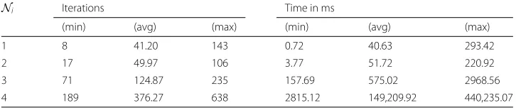
Table 1Performance indicators of the Negative Cycle Algorithm, where Columns 2 to 4 represent numbers of iterations and Columns 5 to 7 show the running times in milliseconds
Ni Iterations Time in ms
(min) (avg) (max) (min) (avg) (max)
1 8 41.20 143 0.72 40.63 293.42
2 17 49.97 106 3.77 51.72 220.92
3 71 124.87 235 157.69 575.02 2968.56
Those instances, for which theMILPprovides better solutions, show that there are non-optimal feasible flows that are not further improvable by our algorithm. Such a flow can be seen as a local minimum for our heuristic. To escape these local minima there are multiple viable strategies. One way could be to allow changes that temporarily increase the total costs, e.g., by canceling cycles with small positive total costs if no negative cycle is found—similar to metaheuristics like Simulated Annealing. As another approach we could search for more complex circulations with negative total costs in the residual graph, e.g., two cycles that share an edge, and cancel those. From a more theoretical standpoint, it would be very interesting to see if optimality can be achieved by identifying only a small set of more complex circulations.
So far, we restricted our heuristic to a single initialization strategy, namely breadth-first search. Other techniques might influence the trajectory of canceling negative cycles and therefore our heuristic might converge to other local minima.
Since our heuristic finds good solution within a short period of time, it might be interesting to see how those solutions can help the MILPto solve WCP. More specifi-cally, a solution given by our algorithm can be given to the solver as an initial feasible solution from which the optimization procedure can be started (warm start). Then, the performances of theMILPwith warm and with cold start can be compared in further simulations.
In our model, it is not required that every turbine has only one edge with outgoing flow. When applying AC-flow or its DC-approximation including phase angles at vertices, it might be desirable to prohibit splitting flow at vertices. In the existing literature, requiring unsplittable flow is often neglected to reduce the complexity of the problem. In terms of future work, allowing only one edge per turbine with outgoing flow in our heuristic seems to be possible by suitably modifying the residual graph and the residual costs. With that, we hope that our model represents real-world wind farms more realistically.
Abbreviations
AC: Alternating current; CMST: CAPACITATEDMINIMUMSPANNINGTREE; DC: Direct current; EU28: the 28 member countries of the European Union; ILP: INTEGERLINEARPROGRAM; MILP: MIXED-INTEGERLINEARPROGRAM; WCP: WINDFARMCABLING PROBLEM
Funding
This work was funded (in part) by the Helmholtz Program Storage and Cross-linked Infrastructures, Topic 6 Superconductivity, Networks and System Integration, and by the Helmholtz future topic Energy Systems Integration. Publication costs for this article were sponsored by the Smart Energy Showcases - Digital Agenda for the Energy Transition (SINTEG) programme.
Availability of data and materials
Benchmark sets are publicly available as stated in Lehmann et al. (2017).
About this Supplement
This article has been published as part ofEnergy InformaticsVolume 1 Supplement 1, 2018: Proceedings of the 7th DACH+ Conference on Energy Informatics. The full contents of the supplement are available online athttps:// energyinformatics.springeropen.com/articles/supplements/volume-1-supplement-1.
Authors’ contributions
DW introduced the topic of wind farm layout and provided overall supervision and guidance. TU contributed general ideas and theoretical insights on negative cycle canceling. SG, FW, and MW implemented and evaluated the algorithms and wrote the article. All authors discussed the results and commented on the manuscript. All authors have approved the final text.
Competing interests
The authors declare that they have no competing interests.
Publisher’s Note
Published: 10 October 2018
References
Berzan C, Veeramachaneni K, McDermott J, O’Reilly U (2016) Algorithms for cable network design on large-scale wind farms.http://thirld.com/files/msrp_techreport.pdf. Accessed 4 Jan 2016
Bellman R (1958) On a routing problem. Q Appl Math 16:87–90.https://doi.org/10.1090/qam/102435
Cerveira A, Baptista J, Solteiro Pires EJ (2014) Optimization design in wind farm distribution network. In: Herrero Á, Baruque B, Klett F, Abraham A, Snášel V, de Carvalho CPLFA, Bringas PG, Zelinka I, Quintián H, Corchado E (eds). International Joint Conference SOCO’13-CISIS’13-ICEUTE’13. Springer International Publishing. ISBN
978-3-319-01854-6, Cham. pp 109–119
de Souza MC, Mahey P, Gendron B (2008) Cycle-based algorithms for multicommodity network flow problems with separable piecewise convex costs. Networks 51(2):133–141.https://doi.org/10.1002/net.20208
Dahmani O, Bourguet S, Machmoum M, Guerin P, Rhein P, Josse L (2015) Optimization of the connection topology of an offshore wind farm network. IEEE Syst J 9:1519–1528
European Commission (2018) 2030 Energy Strategy. https://ec.europa.eu/energy/en/topics/energy-strategy-and-energy-union/2030-energy-strategy. Accessed 31 May 2018
European Commission DG ENER Unit A4 (2018) Energy datasheets: EU28 countries.https://ec.europa.eu/energy/sites/ ener/files/documents/countrydatasheets_feb2018.xlsx. Accessed 31 May 2018
Ford LR, Fulkerson Jr., Fulkerson DR (2010) Flows in Networks. Princeton University Press, New Jersey
Gabrel V, Knippel A, Minoux M (1999) Exact solution of multicommodity network optimization problems with general step cost functions. Oper Res Lett 25(1):15–23. ISSN 0167-6377.https://doi.org/10.1016/S0167-6377(99)00020-6
Goldberg AV, Tarjan RE (1989) Finding minimum-cost circulations by canceling negative cycles. J ACM 36(4):873–886. ISSN 0004-5411.https://doi.org/10.1145/76359.76368
Gupta A, Könemann J (2011) Approximation algorithms for network design: A survey. Sur Oper Res Manag Sci 16(1):3–20. ISSN 1876-7354.https://doi.org/10.1016/j.sorms.2010.06.001
Gurobi optimizer reference manual (2018) Gurobi Optimization, Inc.http://www.gurobi.com. Accessed 31 May 2018 Hornsea Project Three Offshore Wind Farm (2018) 4C Offshore Ltd.
https://www.4coffshore.com/windfarms/hornsea-project-three-united-kingdom-uk1k.html. Accessed 31 May 2018
Klein M (1967) A primal method for minimal cost flows with applications to the assignment and transportation problems. Manag Sci 14(3):205–220.https://doi.org/10.1287/mnsc.14.3.205
Lehmann S, Rutter I, Wagner D, Wegner F (2017) A simulated-annealing-based approach for wind farm cabling. In: Proceedings of the Eighth International Conference on Future Energy Systems, e-Energy ’17. ISBN 978-1-4503-5036-5. ACM, New York. pp 203–215.https://doi.org/10.1145/3077839.3077843
Lumbreras S, Ramos A (2013) Optimal design of the electrical layout of an offshore wind farm applying decomposition strategies. IEEE Transactions on Power Systems 28(2):1434–1441. ISSN 0885-8950.https://doi.org/10.1109/TPWRS. 2012.2204906
Ouorou A, Mahey P (2000) A minimum mean cycle cancelling method for nonlinear multicommodity flow problems. Eur J Oper Res 121(3):532–548. ISSN 0377-2217.https://doi.org/10.1016/S0377-2217(99)00050-8
Radzik T, Goldberg AV (1994) Tight bounds on the number of minimum-mean cycle cancellations and related results. Algorithmica 11(3):226–242. ISSN 1432-0541.https://doi.org/10.1007/BF01240734
Salman FS, Cheriyan J, Ravi R, Subramanian S (2001) Approximating the single-sink link-installation problem in network design. SIAM J Optim 11(3):595–610.https://doi.org/10.1137/S1052623497321432
Santos VP, António Sarmento JNA, Alves M (2014) Offshore wind farm layout optimization – state of the art. J Ocean Wind Energy 1(1):23–29
Shirshak K, Nandigam D, Nandigam M (2017) Design of electrical layout of offshore wind farms. J Renew Sust Energ 9(4):043303.https://doi.org/10.1063/1.4995272
WindEurope asbl/vzw (2018) Wind in power 2017.https://windeurope.org/wp-content/uploads/files/about-wind/ statistics/WindEurope-Annual-Statistics-2017.pdf. Accessed 31 May 2018
Zhao M, Chen Z, Blaabjerg F (2004) Optimization of electrical system for a large DC offshore wind farm by genetic algorithm. In: Proceedings of NORPIE 2004. EPE Association, Brussels. pp 1–8
Submit your manuscript to a
journal and benefi t from:
7 Convenient online submission
7 Rigorous peer review
7 Immediate publication on acceptance
7 Open access: articles freely available online
7 High visibility within the fi eld
7 Retaining the copyright to your article