R E G U L A R A R T I C L E
Open Access
Sentiment analysis methods for
understanding large-scale texts: a case for
using continuum-scored words and word
shift graphs
Andrew J Reagan
1*, Christopher M Danforth
1, Brian Tivnan
2, Jake Ryland Williams
3and
Peter Sheridan Dodds
1*Correspondence:
1University of Vermont, 85 South
Prospect St, Burlington, VT 05405, USA
Full list of author information is available at the end of the article
Abstract
The emergence and global adoption of social media has rendered possible the real-time estimation of population-scale sentiment, an extraordinary capacity which has profound implications for our understanding of human behavior. Given the growing assortment of sentiment-measuring instruments, it is imperative to understand which aspects of sentiment dictionaries contribute to both their
classification accuracy and their ability to provide richer understanding of texts. Here, we perform detailed, quantitative tests and qualitative assessments of 6
dictionary-based methods applied to 4 different corpora, and briefly examine a further 20 methods. We show that while inappropriate for sentences,
dictionary-based methods are generally robust in their classification accuracy for longer texts. Most importantly they can aid understanding of texts with reliable and meaningful word shift graphs if (1) the dictionary covers a sufficiently large portion of a given text’s lexicon when weighted by word usage frequency; and (2) words are scored on a continuous scale.
Keywords: sentiment; sentiment analysis; sentiment dictionaries; language; natural language processing; data visualization; text visualization
1 Introduction
As we move further into what might be called the Sociotechnocene — with increasingly more interactions, decisions, and impact being made by globally distributed people and algorithms — the myriad human social dynamics that have shaped our history have be-come far more visible and measurable than ever before. Of the many ways we are now able to characterize social systems in microscopic detail, sentiment detection for pop-ulations at all scales has become a prominent research arena. Attempts to leverage on-line expression for sentiment mining include prediction of stock markets [–], assessing responses to advertising, real-time monitoring of global happiness [], and measuring a health-related quality of life []. The diverse set of instruments produced by this work now provide indicators that help scientists understand collective behavior, inform pub-lic popub-licy makers, and, in industry, gauge the sentiment of pubpub-lic response to marketing
campaigns. Given their widespread usage and potential to influence social systems, un-derstanding how these instruments perform and how they compare with each other has become imperative. Benchmarking both their ability to provide insight into sentiment and their classification performance focuses future development and provides practical advice to non-experts in selecting a sentiment dictionary.
We identify sentiment detection methods as belonging to one of three categories, each carrying their own advantages and disadvantages:
Dictionary-based methods [, –], Supervised learning methods [], and Unsupervised (or deep) learning methods [].
Here, we focus on dictionary-based methods, which all center around the determina-tion of a textT’s average happiness (sometimes referred to asvalence) with sentiment dictionaryDthrough the equation:
hTD=
w∈DhD(w)·fT(w)
w∈DfT(w)
=
w∈D
hD(w)·pT(w), ()
where we denote each of the words in a given sentiment dictionaryDasw, word senti-ment scores ashD(w), word frequency asfT(w), and normalized frequency ofwinT as
pT(w) =fT(w)/w∈DfT(w). In this way, we measure the happiness of a text in a manner analogous to taking the temperature of a room. While other simple sentiment metrics may be considered, we will see that analyzing individual word contributions is important and that this equation allows for a straightforward, meaningful interpretation.
Dictionary-based methods offer two distinct advantages which we find necessary: () they are in principle corpus agnostic (applicable to corpora without ground truth data available) and () in contrast to black box (highly non-linear) methods, they offer the ability to ‘look under the hood’ at words contributing to a particular score through
word shift graphs(defined fully later; see also [, ]). Indeed, if we are concerned with understanding why a particular scoring method varies — e.g., our undertaking is scien-tific — then word shift graphs are essential tools. In the absence of word shift graphs, or similar devices, explanations of sentiment trends can and often will miss crucial informa-tion.
section of the New York Times. This kind of contextual error is something we can readily identify and correct for through word shift graphs, but could remain hidden to users of nonlinear learning methods.
We lay out our paper as follows. We list and describe the dictionary-based methods we consider in Section ., and outline the corpora we use for tests in Section .. We present our results in Section , comparing all methods in how they perform for specific analyses of the New York Times (NYT) (Section .), movie reviews (Section .), Google Books (Section .), and Twitter (Section .). In Section ., we make some basic comparisons between dictionary-based methods and machine learning approaches. We provide con-cluding remarks in Section and bolster our findings with figures, tables, and additional analysis in the Supplementary Material (supplied as Additional file ).
2 Sentiment dictionaries, corpora, and word shift graphs 2.1 Sentiment dictionaries
The words ‘sentiment dictionary,’ ‘lexicon,’ and ‘corpus’ are often used interchangeably, and for clarity we define our usage as follows.
Sentiment Dictionary Set of words (possibly including word stems) with ratings. Corpus Collection of texts which we seek to analyze.
Lexicon The words contained within a corpus (often said to be ‘tokenized’).
We test the following six sentiment dictionaries in depth:
labMT language assessment by Mechanical Turk []. ANEW Affective Norms of English Words [].
WK Warriner and Kuperman rated words from SUBTLEX by Mechanical Turk [].
MPQA The Multi-Perspective Question Answering (MPQA) Subjectivity Dictio-nary [].
LIWC{,,} Linguistic Inquiry and Word Count, three versions []. OL Opinion Lexicon, developed by Bing Liu [].
We also make note of other sentiment dictionaries:
PANAS-X The Positive and Negative Affect Schedule Expanded [].
Pattern A web mining module for the Python programming language, version . [].
SentiWordNet WordNet synsets each assigned three sentiment scores: positivity, negativ-ity, and objectivity [].
AFINN Words manually rated–to with impact scores by Finn Nielsen []. GI General Inquirer: database of words and manually created semantic and
cognitive categories, including positive and negative connotations []. WDAL Whissel’s Dictionary of Affective Language: words rated in terms of their
Pleasantness, Activation, and Imagery (concreteness) [].
EmoLex NRC Word-Emotion Association Lexicon: emotions and sentiment evoked by common words and phrases using Mechanical Turk [].
HashtagSent NRC Hashtag Sentiment Lexicon: created from Tweets using Pairwise Mu-tual Information with sentiment hashtags as positive and negative labels (here we use only the unigrams) [].
SentLex NRC Sentiment Lexicon: created from the ‘sentiment’ corpus of Tweets, using Pairwise Mutual Information with emoticons as positive and negative labels (here we use only the unigrams) [].
SOCAL Manually constructed general-purpose sentiment dictionary []. SenticNet Sentiment dataset labeled with semantics and dimensions of emotions by
Cambriaet al., version [].
Emoticons Commonly used emoticons with their positive, negative, or neutral emo-tion [].
SentiStrength an API and Java program for general purpose sentiment detection (here we use only the sentiment dictionary) [].
VADER method developed specifically for Twitter and social media analysis []. Umigon Manually built specifically to analyze Tweets from the sentiment
cor-pus [].
USent set of emoticons and bad words that extend MPQA []. EmoSenticNet extends SenticNet words with WNA labels [].
All of these sentiment dictionaries were produced by academic groups, and with the exception of LIWC, they are provided free of charge. In Table , we supply the main as-pects — such as word count, score type (continuum or binary), and license information — for the sentiment dictionaries listed above. In the GitHub repository associated with our paper, https://github.com/andyreagan/sentiment-analysis-comparison, we include all of the sentiment dictionaries except LIWC.
The labMT, ANEW, and WK sentiment dictionaries have scores ranging on a continuum from (low happiness) to (high happiness) with as neutral, whereas the others we test in detail have scores of±, and either explicitly or implicitly (neutral). We will refer to the latter sentiment dictionaries as being binary, even if neutral is included. Other non-binary ranges include a continuous scale from – to (SentiWordNet), integers from – to (AFINN), continuous from to (GI), and continuous from – to (NRC). For coverage tests, we include all available words, to gain a full sense of the breadth of each sentiment dictionary. In scoring, we do not include neutral words from any sentiment dictionary.
We test the labMT, ANEW, and WK dictionaries for a range of stop words (starting with the removal of words scoring withinh= of the neutral score of ) []. The ability to
remove stop words — a common practice for text pre-processing — is one advantage of dictionaries that have a range of scores, allowing us to tune the instrument for maximum performance, while retaining all of the benefits of a dictionary method. We will show that, in agreement with the original paper introducing labMT and looking at Twitter data, a
h= is a pragmatic choice [].
Table 1 Summary of dictionary attributes used in sentiment measurement instruments. We provide all acronyms and abbreviations and further information regarding sentiment dictionaries in Section 2.1. We test the first 6 dictionaries extensively. The range indicates whether scores are continuous or binary (we use the term binary for sentiment dictionaries for which words are scored as±1 and optionally 0).
Dictionary # Entries Range Construction License Ref.
labMT 10,222 1.3→8.5 Survey: MT, 50 ratings CC [5]
ANEW 1,034 1.2→8.8 Survey: UF Intro Psych Free for research [7]
LIWC07 4,483 [–1, 0, 1] Manual Paid, commercial [8]
MPQA 7,192 [–1, 0, 1] Manual + ML GNU GPL [9]
OL 6,782 [–1, 1] Dictionary propagation Free [10]
WK 13,915 1.3→8.5 Survey: MT, 14-18 ratings CC [11]
LIWC01 2,322 [–1, 0, 1] Manual Paid, commercial [8]
LIWC15 6,549 [–1, 0, 1] Manual Paid, commercial [8]
PANAS-X 20 [–1, 1] Manual Copyrighted paper [17]
Pattern 1,528 –1.0→1.0 Unspecified BSD [18]
SentiWordNet 147,700 –1.0→1.0 Synset synonyms CC BY-SA 3.0 [19]
AFINN 2,477 [–5, –4,. . ., 4, 5] Manual ODbL v1.0 [20]
GI 3,629 [–1, 1] Harvard-IV-4 Unspecified [21]
WDAL 8,743 0.0→3.0 Survey: Columbia students Unspecified [22]
EmoLex 14,182 [–1, 0, 1] Survey: MT Free for research [23]
MaxDiff 1,515 –1.0→1.0 Survey: MT, MaxDiff Free for research [24] HashtagSent 54,129 –6.9→7.5 PMI with hashtags Free for research [25] Sent140Lex 62,468 –5.0→5.0 PMI with emoticons Free for research [26]
SOCAL 7,494 –30.2→30.7 Manual GNU GPL [27]
SenticNet 30,000 –1.0→1.0 Label propogation Citation requested [28]
Emoticons 132 [–1, 0, 1] Manual Open source code [29]
SentiStrength 2,615 [–5, –4,. . ., 4, 5] LIWC + GI Free for research [30] VADER 7,502 –3.9→3.4 MT survey, 10 ratings Freely available [31]
Umigon 927 [–1, 1] Manual Public Domain [32]
USent 592 [–1, 1] Manual CC [33]
EmoSenticNet 13,188 [–10, –2, –1, 0, 1, 10] Bootstrapped extension Non-commercial [34]
2.2 Corpora tested
For each sentiment dictionary, we test both the coverage and the ability to detect previ-ously observed and/or known patterns within each of the following corpora, noting the pattern we hope to discern:
The New York Times (NYT) []: Goal of understanding differences between sections and ranking by sentiment (Section .).
Movie reviews []: Goal of discerning how emotional language differs in positive and negative reviews and how these differences influence classification accuracy
(Section .).
Google Books []: Goal of understanding time series (Section .). Twitter: Goal of understanding time series (Section .).
For the corpora other than the movie reviews and small numbers of tagged Tweets, there is no publicly available ground truth sentiment, so we instead make comparisons between methods and examine how words contribute to scores. We note that measuring how pat-terns of sentiment compare with societal measures of well being would also be possible []. We offer greater detail on corpus processing below, and we also provide the relevant scripts on GitHub at https://github.com/andyreagan/sentiment-analysis-comparison.
2.3 Word shift graphs
sentiment analysis as a lens that allows us to see how the emotive words in a text shape the overall content. This is accomplished by first analyzing each word to find its individual contribution to the difference in sentiment scores between two texts. The most important and final step is to examine the words themselves, ranked by their individual contribution. Of the four corpora that we analyze, three rely on this type of qualitative analysis: using the sentiment dictionary as a tool to better understand the sentiment of the corpora rather than as a binary classifier.
To make this possible, we must first find the contribution of each word individually. Starting with the ANEW sentiment dictionary and two texts which we label reference and comparison, we take the difference of their sentiment scoresh(comp)ANEWandh(ref )ANEW, rearrange terms, and arrive at
hcompANEW–hrefANEW=
w∈ANEW
hANEW(w) –hrefANEW
+/–
pcomp(w) –pref(w)
↑/↓
.
Each wordwin the summation contributes to the sentiment difference between the texts according to () its sentiment relative to the reference text (+/– = more/less positive), and () its change in frequency of usage (↑/↓= more/less frequent). As a first step, it is possible to visualize this sorted word list in a table, along with the basic indicators of how its contribution is constituted. We use word shift graphs to present this informa-tion in the most accessible manner to advanced users. For further detail, we refer the reader to our instructional post and video at http://www.uvm.edu/storylab//// hedonometer---measuring-happiness-and-using-word-shifts/.
3 Results
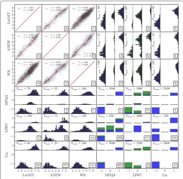
In Figure , we show a direct comparison between word scores for each pair of the dictio-naries tested. Overall, we find strong agreement between all dictiodictio-naries with the excep-tions we note below. As a guide, we will provide more detail on the individual comparison between the labMT dictionary and the other five dictionaries by examining the words whose scores disagree across dictionaries shown in Figure . We refer the reader to the S Appendix for the remaining individual comparisons.
To start with, consider the comparison of the labMT and ANEW dictionaries on a word-for-word basis. Because these dictionaries share the same range of values, a scatterplot is the natural way to visualize the comparison. Across the top row of Figure , which com-pares labMT to the other dictionaries, we see in Panel B for the labMT-ANEW compar-ison that the RMA best fit [] is
hlabMT(w) = .∗hANEW(w) + .
Figure 1 Direct comparison of the words in each of the dictionaries tested.For the comparison of two dictionaries, we plot words that are matched by the independent variable ‘x’ in the dependent variable ‘y’. Because of this, and cross stem matching, the plots are not symmetric across the diagonal of the entire figure. Where the scores are continuous in both dictionaries, we compute the RMA linear fit. When a sentiment dictionary contains both fixed and stem words, we plot the matches by fixed words in blue and by stem words in green. The axes in the bar plots are not of the same height, due to large mismatches in the number of words in the dictionaries, and we note the maximum height of the bar in the upper left of such plots. Detailed analysis of Panel C can be found in [39]. We provide a table for each off-diagonal panel in the S2 Appendix with the words whose scores exhibit the greatest mismatch, and a subset of these tables in Figure 2.
Comparing labMT with WK in Panel C of Figure , we again find a fit with slope near , and with a smaller positive shift:hlabMT(w) = .∗hWK(w) + .. The words farthest
from the best fit line, shown in Panel B of Figure , are (labMT, WK): sue (., .), boogie (., .), exclusive (., .), wake (., .), federal (., .), stroke (., .), gay (., .), patient (., .), user (., .), and blow (., .). Like labMT, the WK dictionary used a Mechanical Turk online survey to gather word ratings. We speculate that the variation may in part be due to differences in the number of scores required for each word in the surveys, with - in WK and in labMT. For an in depth comparison of these sentiment dictionaries, see reference [].
with-Figure 2 The specific words from Panels G, M, S and Y of with-Figure 1 with the greatest mismatch.Only the center histogram from Panel Y of Figure 1 is included. We emphasize that the labMT dictionary scores generally agree well with the other dictionaries, and we are looking at the marginal words with the strongest disagreement. Within these words, we detect differences in the creation of these dictionaries that carry through to these edge cases. Panel A: The words with most different scores between the labMT and ANEW dictionaries are suggestive of the different meanings that such words entail for the different demographic surveyed to score the words. Panel B: Both dictionaries use surveys from the same demographic (Mechanical Turk), where the labMT dictionary required more individual ratings for each word (at least 50, compared to 14) and appears to have dampened the effect of multiple meaning words. Panels C-E: The words in labMT matched by MPQA with scores of –1, 0, and +1 in MPQA show that there are at least a few words with negative rating in MPQA that are not negative (including the happiest word in the labMT dictionary: ‘laughter’), not all of the MPQA words with score 0 are neutral, and that MPQA’s positive words are mostly positive according to the labMT score. Panel F: The function words in the expert-curated LIWC dictionary are not emotionally neutral.
out stems (blue) than those with stems (green), and that each score in –, , + from MPQA corresponds to a wider range of scores in labMT. We examine the shared indi-vidual words from labMT with high sentiment scores and MPQA with score –, both the happiest and the least happy in labMT with MPQA score , and the least happy when MPQA is (Figure Panels C-E). The happiest words in labMT matched by MPQA words with score – are: moonlight (.), cutest (.), finest (.), funniest (.), comedy (.), laughs (.), laughing (.), laugh (.), laughed (.), laugh-ter (.). This is an immediately troubling list of evidently positive words rated as – in MPQA. We observe the top are matched by the stem ‘laugh*’ in MPQA. The least happy words and happiest words in labMT matched by words in MPQA with score are: sorrows (.), screaming (.), couldn’t (.), pressures (.), couldnt (.), and baby (.), precious (.), strength (.), surprise (.), and song (.). We see that these MPQA word scores are departures from the other dictionaries, warranting further concern. The least happy words in labMT with score + in MPQA that are matched by MPQA are: vulnerable (.), court (.), sanctions (.), defendant (.), conviction (.), backwards (.), courts (.), defendants (.), court’s (.), and correction (.).
ex-amine words contributing to overall sentiment. We note again that the use of word shift graphs of some kind would have exposed these problematic scores immediately.
For the labMT-LIWC comparison in Panel E of Figure we examine the same matched word lists as before. The happiest words in labMT matched by words in LIWC with score – are: trick (.), shakin (.), number (.), geek (.), tricks (.), defence (.), dwell (.), doubtless (.), numbers (.), shakespeare (.). From Panel F of Figure , the least happy neutral words and happiest neutral words in LIWC, matched in LabMT from LIWC words (i.e., using the word stems in LIWC to match across LabMT, directionality matters), are: negative (.), lack (.), couldn’t (.), cannot (.), never (.), millions (.), couple (.), million (.), billion (.), millionaire (.). The least happy words in labMT with score + in LIWC that are matched by LIWC are: mer-rill (.), richardson (.), dynamite (.), careful (.), richard (.), silly (.), gloria (.), securities (.), boldface (.), treasury’s (.). The + and – words in LIWC match some neutral words in labMT, which is not alarming. However, the problems with the ‘neutral’ words in the LIWC set are evident: these are not emotionally neutral words [].
For the labMT-OL comparison in Panel E of Figure we again examine the same matched word lists as before (except the neutral word list because OL has no explicit neutral words). The happiest words in labMT matched by OL’s negative list are: myth (.), puppet (.), skinny (.), jam (.), challenging (.), fiction (.), lemon (.), tenderness (.), joke (.), funny (.). The least happy words in labMT with score + in OL that are matched by OL are: defeated (.), defeat (.), envy (.), ob-session (.), tough (.), dominated (.), unreal (.), striking (.), sharp (.), sensitive (.). Despite nearly twice as many negative words in OL as positive words (at odds with the frequency-dependent positivity bias of language []), after examining the words which are the most differently scored and seeing how quickly the labMT scores move into the neutral range, we can conclude that these dictionaries generally agree with the exception of only a few bad matches.
Our direct comparisons between the word scores in sentiment dictionaries, while per-haps tedious, have brought to light many problematic word scores. Our analysis also serves as a template for further comparisons of the words across new sentiment dictionaries. The six sentiment dictionaries under careful examination in the present study are further an-alyzed in the Supporting Information. Next, we examine how each sentiment dictionary can aid in understanding the sentiments contained in articles from the New York Times.
3.1 New York Times word shift analysis
The New York Times corpus [] is split into sections of the newspaper that are roughly contiguous throughout the data from -. With each sentiment dictionary, we rate each section and then compute word shift graphs (described below) against the baseline, and produce a happiness ranked list of the sections.
To gain understanding of the sentiment expressed by any given text relative to another text, it is necessary to inspect the words which contribute most significantly by their emotional strength and the change in frequency of usage. We do this through the use of word shift graphs, which plot the percentage contribution of each wordwfrom the sentiment dictionary (denotedδhANEW(w)) to the shift in average happiness between two
analyze a single text and to compare two texts, here focusing on comparing text within corpora. For a derivation of the algorithm used to make word shift graphs while separat-ing the frequency and sentiment information, we refer the reader to Equations and in []. We consider both the sentiment difference and frequency difference components of
δhANEW(w) by writing each term of Eq. () as in []:
δhANEW(w) =
hANEW(w) –hrefANEW
hcompANEW–hrefANEW
p(w)comp–p(w)ref. ()
An in-depth explanation of how to interpret the word shift graph can also be found at http://hedonometer.org/instructions.html#wordshifts.
To both demonstrate the necessity of using word shift graphs in carrying out sentiment analysis, and to gain understanding about the ranking of New York Times sections by each sentiment dictionary, we look at word shift graphs for the ‘Society’ section of the news-paper from each sentiment dictionary in Figure , with the reference text being the whole of the New York Times. The ‘Society’ section happiness ranks , , , , , and within the happiness of each of the sections in the dictionaries labMT, ANEW, WK, MPQA, LIWC, and OL, respectively. These graphs show only the very top of the distributions which range in length from , (ANEW) to , words (WK).
First, using the labMT dictionary, we see that the words ‘graduated’, ‘father’, and ‘univer-sity’ top the list, which is dominated by positive words that occur more frequently (+↑). These more frequent positive words paint a clear picture of family life (relationships, wed-dings, and divorces), as well as university accomplishment (graduations and college). In general, we are able to observe with only these words that the ‘Society’ section is where we find the details of these events.
From the ANEW dictionary, we see that a few positive words have increased frequency, lead by ‘mother’, ‘father’, and ‘bride’. Looking at this shift in isolation, we see only these words with three more (‘graduate’, ‘wedding’, and ‘couple’) that would lead us to suspect these topics are present in the ‘Society’ section.
The WK dictionary, with the most individual word scores of any sentiment dictionary tested, agrees with labMT and ANEW that the ‘Society’ section is the happiest section, with a somewhat similar set of words at the top: ‘new’, ‘university’, and ‘father’. Low coverage of the New York Times corpus (see Figure S) resulted in less specific words describing the ‘Society’ section, with more words that go down in frequency in the shift. With the words ‘bride’ and ‘wedding’ up, as well as ‘university’, ‘graduate’, and ‘college’, it is evident that the ‘Society’ section covers both graduations and weddings, in consensus with the other sentiment dictionaries.
The MPQA dictionary ranks the ‘Society’ section th of the NYT sections, a de-parture from the other rankings, with the words ‘mar*’, ‘retire*’, and ‘yes*’ the top three contributing words (where ‘*’ denotes a wildcard ‘stem’ match). Negative words increas-ing in frequency (–↑) are the most common type near the top, and of these, the words with the biggest contributions are being scored incorrectly in this context (specifically words ‘mar*’, ‘retire*’, ‘bar*’, ‘division’, and ‘miss*’). Looking more in depth at the problems created by the first out of context word match, we find , unique words match ‘mar*’. The five most frequent, with counts in parenthesis, are married (,), marriage (,), mar-keting (,), mary (,), and mark (,). The score for these words in MPQA is –, in stark contrast to the scores in other sentiment dictionaries (e.g., the labMT scores are ., ., ., ., and .). These problems plague the MPQA dictionary for scoring the New York Times corpus, and without using word shift graphs would have gone completely unseen. In an attempt to fix contextual issues by fixing corpus-specific words, we remove ‘mar*’, ‘retire*’, ‘vice’, ‘bar*’, and ‘miss*’ and find that the MPQA dictionary ranks the Society section of the NYT at th of the sections.
have seen. Nevertheless, LIWC finds consensus with the ‘Society’ section ranked the top section, due in large part to a lack of negative words ‘war’ (rank ) and ‘fight*’ (rank ). The OL sentiment dictionary departs from the consensus and ranks the ‘Society’ section at th out of the sections. The top three words, ‘vice’, ‘miss’, and ‘concern’, contribute largely with respect to the rest of distribution, of which two are clearly being used in the wrong sense. For a more reasonable analysis we remove both ‘vice’ and ‘miss’ from the OL dictionary to score this text, and in doing so the happiness goes from . to ., making the ‘Society’ section the second happiest of the sections. Focusing on the words, we see that the OL dictionary finds many positive words increasing in frequency (+↑) that are mostly generic. In the word shift graph we do not find the wedding or university events as in sentiment dictionaries with more coverage, but rather a variety of positive language surrounding these events, for example, ‘works’ (), ‘benefit’ (), ‘honor’ (), ‘best’ (), ‘great’ (), ‘trust’ (), ‘love’ (), etc. While this does not provide insight into the topics, the OL sentiment dictionary with fixes from the word shift graph analysis does provide details on the emotive words that make the ‘Society’ section one of the happiest sections.
In conclusion, we find that of the dictionaries score the ‘Society’ section at number , and in these cases we use the word shift graph to uncover the nuances of the language used. We find, unsurprisingly, that the most matches are found by the labMT dictionary, which is in part built from the NYT corpus (see S Appendix for coverage plots). Without as much corpus-specific coverage, we note that while the specifies of the text remain hidden, the LIWC and OL dictionaries still highlight the positive language in this section. Of the two that did not score the ‘Society’ section at the top, we are able to assess and repair the MPQA and the OL dictionaries by removing the words ‘mar*’, ‘retire*’, ‘vice*’, ‘bar*’, ‘miss*’ and ‘vice’, and ‘miss’, respectively. By identifying words used in the wrong sense/context using the word shift graph, we directly improve the sentiment score for the New York Times corpus from both MPQA and OL dictionaries closer to consensus. While the OL dictionary, with two corrections, agrees with the other dictionaries, the MPQA dictionary with five corrections still ranks the Society section of the NYT as the th happiest of the sections.
In the first Figure in S Appendix we show scatterplots for each comparison, and com-pute the Reduced Major Axes (RMA) regression fit []. In the second Figure in S Ap-pendix we show the sorted bar chart from each sentiment dictionary.
3.2 Movie reviews classification and word shift graph analysis
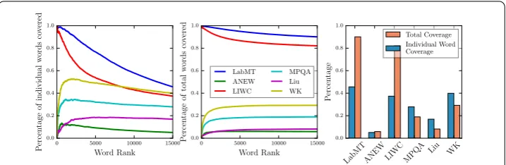
Figure 4 Coverage of the words in the movie reviews by each of the dictionaries.We observe that the labMT dictionary has the highest coverage of words in the movie reviews corpus both across word rank and cumulatively. The LIWC dictionary has initially high coverage since it contains some high-frequency function words, but quickly drops off across rank. The WK dictionary coverage increases across word rank and cumulatively, indicating that it contains a large number of less common words in the movie review corpus. The OL, ANEW, and MPQA have a cumulative coverage of less than 20% of the lexicon.
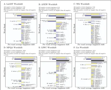
To analyze which words are being used by each sentiment dictionary, we compute word shift graphs of the entire positive corpus versus the entire negative corpus in Figure . Across the board, we see that a decrease in negative words is the most important word type for each sentiment dictionary, with the word ‘bad’ being the top word for every sentiment dictionary in which it is scored (ANEW does not have it). Other observations that we can make from the word shift graphs include a few words that are potentially being used out of context: ‘movie’, ‘comedy’, ‘plot’, ‘horror’, ‘war’, ‘just’.
In the lower right panel of Figure , the percentage overlap of positive and negative review distributions presents us with a simple summary of sentiment dictionary perfor-mance on this tagged corpus. The ANEW dictionary stands out as being considerably less capable of distinguishing positive from negative. In order, we then see WK is slightly better overall, labMT and LIWC perform similarly better than WK overall, and then MPQA and OL are each a degree better again, across the review lengths (see below for hard numbers at review length). Two Figures in the S Appendix show the distributions for review and for combined reviews.
Classifying single reviews as positive or negative, the F-scores are: labMT ., ANEW ., LIWC ., MPQA ., OL ., and WK . (see Table S). We roughly confirm a rule-of-thumb that , words are enough to score with a sentiment dictionary con-fidently, with all dictionaries except MPQA and ANEW achieving % accuracy with this many words. We sample the number of reviews evenly in log space, generating sets of re-views with average word counts of ,, ,, ,, ,, and , words. Specifi-cally, the number of reviews necessary to achieve % accuracy is reviews (, words) for labMT, reviews (, words) for ANEW, reviews (, words) for LIWC, reviews (, words) for MPQA, reviews (, words) for OL, and reviews (, words) for WK.
Figure 5 Word shift graphs for the movie review corpus.By analyzing the words that contribute most significantly to the sentiment score produced by each sentiment dictionary we are able to identify words that are problematic for each sentiment dictionary at the word-level, and generate an understanding of the emotional texture of the movie review corpus. Again we find that coverage of the lexicon is essential to produce meaningful word shift graphs, with the labMT dictionary providing the most coverage of this corpus and producing the most detailed word shift graphs. All words on the left hand side of these word shift graphs are words that individually made the positive reviews score more negatively than the negative reviews, and the removal of these words would improve the accuracy of the ratings given by each sentiment dictionary. In particular, across each sentiment dictionary the word shift graphs show that domain-specific words such as ‘war’ and ‘movie’ are used more frequently in the positive reviews and are not useful in determining the polarity of a single review.
an F-score of .. The results for each sentiment dictionary are included in Table S, with an average (median) F score of . (.) across all dictionaries. While these re-sults do cast doubt on the ability to classify positive and negative reviews from single sen-tences using dictionary based methods, we note that we need not expect the sentiment of individual sentences to be strongly correlated with the overall review polarity.
3.3 Google books time series and word shift analysis
We use the Google books dataset with all English books [], from which we remove part of speech tagging and split into years. From this, we make time series by year, and word shift graphs of decades versus the baseline. In addition, to assess the similarity of each time series, we produce correlations between each of the time series.
Figure 6 The score assigned to increasing numbers of reviews drawn from the tagged positive and negative sets.For each sentiment dictionary we show mean sentiment and 1 standard deviation over 100 samples for each distribution of reviews in Panels A-F. For comparison we compute the fraction of the distributions that overlap in Panel G. At the single review level for each sentiment dictionary this simple performance statistic (fraction of distribution overlap) ranks the OL dictionary in first place, the MPQA, LIWC, and labMT dictionaries in a second place tie, WK in fifth, and ANEW far behind. All dictionaries require on the order of 1,000 words to achieve 95% classification accuracy.
Figure 7 Google Books sentiment time series from each sentiment dictionary, with stop values of 0.5, 1.0, and 1.5 from the dictionaries with word scores in the 1-9 range.To normalize the sentiment score, we subtract the mean and divide by the absolute range. We observe that each time series has increased variance, with a few pronounced negative time periods, and trending positive towards the end of the corpus. The score of labMT varies substantially with different stop values, although remaining highly correlated, and finds absolute lows near the World Wars. The LIWC and OL dictionaries trend down towards 1990, dipping as low as the war periods.
In Figure , we plot the sentiment time series for Google Books. Three immediate trends stand out: a dip near the Great Depression, a dip near World War II, and a general upswing in the ’s and ’s. From these general trends, a few dictionaries waver: OL does not dip as much for WW, OL and LIWC stay lower in the ’s and ’s, and labMT with
h= ., . go downward near the end of the ’s. We take a closer look into the ’s
to see what each sentiment dictionary is picking up in Google Books around World War in Figure in S Appendix.
are ‘no’ and ‘great’, and we infer that the word ‘great’ is being seen from mention of ‘The Great Depression’ or ‘The Great War’. All dictionaries but ANEW have ‘great’ in the top words, and each sentiment dictionary could be made more accurate if we remove this word.
In Panel A of the ’s word shift Figure in S Appendix, beyond the top words, in-creasing words are mostly negative and war-related: ‘against’, ‘enemy’, ‘operation’, which we could expect from this time period.
In Panel B, the ANEW dictionary scores the ’s of Google Books lower than the baseline as well, finding ‘war’, ‘cancer’, and ‘cell’ to be the most important three words. With only , words, there is not enough coverage to see anything beyond the top word ‘war,’ and the shift is dominated by words that go down in frequency.
In Panel C, the WK dictionary finds the ’s to be slightly less happy than the baseline, with the top three words being ‘war’, ‘great’, and ‘old’. We see many of the same war-related words as in labMT, as well as some positive words like ‘good’ and ‘be’ are up in frequency. The word ‘first’ could be an artifact of first aid, a claim that could be substantiated with further analysis of the Google Books corpus at the -gram level but beyond the scope of this manuscript.
In Panel D, the MPQA dictionary rates the ’s slightly less happy than the baseline, with the top three words being ‘war’, ‘great’, and ‘differ*’. Beyond the top word ‘war’, the score is dominated by words decreasing in frequency, with only a few words up in frequency. Without specific words increasing in frequency as contextual guides, it is difficult to obtain a good glance at the nature of the text. Once again, having a higher coverage of the words in the corpus enables understanding.
In Panel E, the LIWC dictionary rates the ’s nearly the same as the baseline, with the top three words being ‘war’, ‘great’, and ‘argu*’. When the scores are nearly the same, although the ’s are slightly higher in happiness here, the word shift is a view into how the words of the reference and comparison text vary. In addition to a few war related words being up and bringing the score down (‘fight’, ‘enemy’, ‘attack’), we see some pos-itive words also being up that could also be war related: ‘certain’, ‘interest’, and ‘definite’. Although LIWC does not manage to find World War II as a low point of the th century, the words that contribute to LIWCs score for the ’s compared to all years are useful in understanding the corpus.
In Panel F, the OL dictionary rates the ’s as happier than the baseline, with the top three words being ‘great’, ‘support’, and ‘like’. With positive words up, and negative word up, we see how the OL dictionary misses the war without the word ‘war’ itself and with only ‘enemy’ contributing from the words surrounding the conflict. The nature of the positive words that are up is unclear, and could justify a more detailed analysis of why the OL dictionary fails here.
3.4 Twitter time series analysis
Figure 8 Normalized sentiment time series on Twitter usinghof 1.0 for all dictionaries.To normalize
the sentiment score, we subtract the mean and divide by the absolute range. The resolution is 1 day, and draws on the 10% gardenhose sample of public Tweets provided by Twitter. All of the dictionaries exhibit wide variation for very early Tweets, and from 2012 onward generally track together strongly with the exception of MPQA and LIWC. The LIWC and MPQA dictionaries show opposite trends: a rise until 2012 with a decline after 2012 from LIWC, and a decline before 2012 with a rise afterwards from MPQA. To analyze the trends we look at the words driving the movement across years using word shift Figures in S7 Appendix. An interactive version of this Figure using the labMT dictionary be found at http://hedonometer.org.
Figure 9 Pearson’srcorrelation between daily resolution Twitter sentiment time series for each sentiment dictionary.We see that there is strong agreement within dictionaries, with the biggest differences coming from the stop value of h= 0.5 for labMT and WK. The labMT and OL dictionaries do not strongly disagree with any of the others, while LIWC is the least correlated overall with other dictionaries. labMT and OL correlate strongly with each other, and disagree most with the ANEW, LIWC, and MPQA dictionaries. The two least correlated dictionaries are the LIWC and MPQA dictionaries. Again, since there is no publicly accessible ground truth for Twitter sentiment, we compare dictionaries against the others, and look at
the words. With these criteria, we find the labMT and OL dictionaries to be the most robust with Tweets.
In Figure , we present a daily sentiment time series of Twitter processed using each of the dictionaries being tested. With the exception of LIWC and MPQA we observe that the dictionaries generally track well together across the entire range. A strong weekly cycle is present in all, although muted for ANEW. An interactive version of the plot in Figure can be found at http://hedonometer.org.
We plot the Pearson’s correlation between all time series in Figure , and confirm some of the general observations that we can make from the time series. Namely, the LIWC and MPQA time series disagree the most from the others, and even more so with each other. Generally, we see strong agreement within dictionaries with varying stop valuesh.
negative words going up in frequency (see word shift Figure in Appendix S). All of the dictionaries agree most strongly in , all finding a lot of negative language and swearing that brings scores down (see word shift Figure in Appendix S). From the bottom at , LIWC continues to go downward while the others trend back up. The signal from MPQA jumps to the most positive, and LIWC does start trending back up eventually. We analyze the words in with a word shift against all years of Tweets for each sentiment dictionary in each panel in the word shift Figure in Appendix S: A. labMT scores as less happy with more negative language. B. ANEW finds it happier with a few positive words up. C. WK finds it happier with more negative words (like labMT). D. MPQA finds it more positive with less negative words. E. LIWC finds it less positive with more negative and less positive words. F. OL finds it to be of the same sentiment as the background with a balance in positive and negative word usage. From these word shift graphs, we can analyze which words cause MPQA and LIWC to disagree with the other dictionaries: the disagreement of MPQA is again marred by broad stem matches, and the disagreement of LIWC is due to a lack of coverage.
3.5 Brief comparison to machine learning methods
We implement a Naive Bayes (NB) classifier (sometimes harshly called idiot Bayes []) on the tagged movie review dataset to examine how individual words contribute in ma-chine learning classification. While more advanced methods have better classification ac-curacy, we focus on the simplest example to illustrate how analysis at the individual word level aids in understanding sentiment analysis scores. We use a / split of the data into training and out-of-sample testing sets, and examine the model performance on random permutations of this split. Again following standard best-practice, we remove the top ranked words (‘stop words’) from the , most frequent words, and use the re-maining , words in our classifier for maximum performance (we observe a .% im-provement). Our implementation is analogous to those found in common Python natural language processing packages (see ‘NLTK’ or ‘TextBlob’ in []).
As we should expect, at the level of single review, NB outperforms the dictionary-based methods with a classification accuracy of .-.% averaged over trials. As the num-ber of reviews is increased, the overlap from NB decreases, and using our simple ‘fraction overlapping’ metric, the error drops to with more than reviews. Overall, with Naive Bayes we are able to classify a higher percentage of individual reviews correctly, but with more variance.
In the two Tables in S Appendix we compute the words which the NB classifier uses to classify all of the positive reviews as positive, and all of the negative reviews as positive. The Natural Language Toolkit (NLTK []) implements a method to obtain the ‘most informative’ words, by taking the ratio of the likelihood of words between all available classes, and looking for the largest ratio:
max
all wordsw
P(w|ci)
P(w|cj)
()
for all combinations of classesci,cj. This is possible because of the ‘naive’ assumption that
We find that the trained NB classifier relies heavily on words that are very specific to the training set including the names of actors of the movies themselves, making them useful as classifiers but not in understanding the nature of the text. We report the top words for both positive and negative classes using both the ratio and difference methods in Table in S Appendix. To classify a document using NB, we use the frequency of each word in the document in conjunction with the probability that that word occurred in each labeled classci. While steps can be taken to avoid this type of over-fitting, it is an ever-present
danger that remains hidden without word shift graphs or similar.
We next take the movie-review-trained NB classifier and use it to classify the New York Times sections, both by ranking them and by looking at the words (the above ratio and difference weighted by the occurrence of the words). We ranked the Sections different times, and among those find the ‘Television’ section both by far the happiest, and by far the least happy in independent tests. We show these rankings and report the top words used to score the ‘Society’ section in Table S.
We thus see that the NB classifier, a linear learning method, may perform poorly when assessing sentiment outside of the corpus on which it is trained. In general, performance will vary depending on the statistical dissimilarity of the training and novel corpora. Added to this is the inscrutability of black box methods: while susceptible to the aforementioned difficulty, nonlinear learning methods (unlike NB) also render detailed examination of how individual words contribute to a text’s score more difficult.
4 Conclusion
We have shown that measuring sentiment in various corpora presents unique challenges, and that sentiment dictionary performance is situation dependent. Across the board, the ANEW dictionary performs poorly, and the continued use of this sentiment dictionary with clearly better alternatives is a questionable choice. We have seen that the MPQA dictionary does not agree with the other five dictionaries on the NYT corpus and Twitter corpus due to a variety of context, word sense, phrase, and stem matching issues, and we would not recommend using this sentiment dictionary. While the OL achieves the highest binary classification accuracy, in comparison to labMT, the WK, LIWC, and OL dictionaries fail to provide much detail in corpora where their coverage is lower, including all four corpora tested, the main goal of our analysis. Sufficient coverage is essential for producing meaningful word shift graphs and thereby enabling deeper understanding.
languages of interest. With phrase dictionaries, the resulting phrase shift graphs will al-low for a more nuanced and detailed analysis of a corpus’s sentiment score [], ultimately affording clearer stories for sentiment dynamics.
Additional material
Additional file 1: Supplementary Material.(pdf )
Funding Not applicable.
Abbreviations
NYT, New York Times; MT, Mechanical Turk; ML, Machine Learning; BSD, Berkeley Software Distribution; CC, Creative Commons; GNU, GNU’s Not Unix; GNU GPL, GNU General Public License; RMA, Reduced Major Axes; VACC, Vermont Advanced Computing Core; NB, Naive Bayes; NLTK, Natural Language Toolkit; labMT, language assessment by Mechanical Turk [5]; ANEW, Affective Norms of English Words [7]; WK, Warriner and Kuperman rated words from SUBTLEX by Mechanical Turk [11]; MPQA, The Multi-Perspective Question Answering (MPQA) Subjectivity Dictionary [9]; LIWC{01,07,15}, Linguistic Inquiry and Word Count [8]; OL, Opinion Lexicon, developed by Bing Liu [10]; PANAS-X, The Positive and Negative Affect Schedule Expanded [17]; AFINN, Words manually rated –5 to 5 with impact scores by Finn Nielsen [20]; GI, General Inquirer [21]; WDAL, Whissel’s Dictionary of Affective Language [22]; EmoLex, NRC Word-Emotion Association Lexicon [23]; MaxDiff, NRC MaxDiff Twitter Sentiment Lexicon[24]; HashtagSent, NRC Hashtag Sentiment Lexicon [25]; Sent140Lex, NRC Sentiment140 Lexicon [26]; SOCAL, Semantic Orientation CALculator [27]; VADER, Valence Aware Dictionary for sEntiment Reasoning [31]; USent, set of emoticons and inappropriate words that extend MPQA [33].
Availability of data and materials
In the following GitHub repository associated with our paper, we include all of the sentiment dictionary data (except LIWC). In addition, we also provide the scripts to reproduce our analysis. The repository is publicly available on GitHub at https://github.com/andyreagan/sentiment-analysis-comparison.
Competing interests
The authors declare that they have no competing interests.
Authors’ contributions
AJR, CMD, BT, JRW, and PSD designed research. AJR performed research. JRW contributed analytic tools. AJR, CMD, BT, and PSD analyzed data. AJR, CMD, and PSD wrote the paper. All authors read and approved the final manuscript.
Author details
1University of Vermont, 85 South Prospect St, Burlington, VT 05405, USA.2The MITRE Corporation, 7525 Colshire Drive,
McLean, VA 22102, USA.3Drexel University, 3141 Chestnut Street, Philadelphia, PA 19104, USA.
Publisher’s Note
Springer Nature remains neutral with regard to jurisdictional claims in published maps and institutional affiliations.
Received: 24 January 2017 Accepted: 14 September 2017 References
1. Bollen J, Mao H, Zeng X (2011) Twitter mood predicts the stock market. J Comput Sci 2(1):1-8
2. Si J, Mukherjee A, Liu B, Li Q, Li H, Deng X (2013) Exploiting topic based Twitter sentiment for stock prediction. In: ACL, vol 2, pp 24-29
3. Chung S, Liu S (2011) Predicting stock market fluctuations from Twitter. Berkeley, California
4. Ruiz EJ, Hristidis V, Castillo C, Gionis A, Jaimes A (2012) Correlating financial time series with micro-blogging activity. In: Proceedings of the fifth ACM international conference on web search and data mining. ACM, New York, pp 513-522
5. Dodds PS, Clark EM, Desu S, Frank MR, Reagan AJ, Williams JR, Mitchell L, Harris KD Kloumann IM, Bagrow JP, Megerdoomian K, McMahon MT, Tivnan BF, Danforth CM (2015) Human language reveals a universal positivity bias. Proc Natl Acad Sci USA 112(8):2389-2394
6. Alajajian SE, Williams JR, Reagan AJ, Alajajian SC, Frank MR, Mitchell L, Lahne J, Danforth CM, Dodds PS (2017) The Lexicocalorimeter: gauging public health through caloric input and output on social media. PLoS ONE 12(2):e0168893. doi:10.1371/journal.pone.0168893
7. Bradley MM Lang PJ (1999) Affective norms for english words (ANEW): stimuli, instruction manual and affective ratings. Technical report c-1, University of Florida, Gainesville, FL
8. Pennebaker JW, Francis ME, Booth RJ (2001) Linguistic inquiry and word count: LIWC 2001. Erlbaum, Mahway 9. Wilson T, Wiebe J, Hoffmann P (2005) Recognizing contextual polarity in phrase-level sentiment analysis. In:
Proceedings of human language technologies conference/conference on empirical methods in natural language processing (HLT/EMNLP 2005)
11. Warriner AB, Kuperman V, Brysbaert M (2013) Norms of valence, arousal, and dominance for 13,915 English lemmas. Behav Res Methods 45(4):1191-1207. doi:10.3758/s13428-012-0314-x
12. Socher R, Perelygin A, Wu JY, Chuang J, Manning CD, Ng AY, Potts C (2013) Recursive deep models for semantic compositionality over a sentiment treebank. In: Proceedings of the conference on empirical methods in natural language processing (EMNLP), pp 1631-1642. Citeseer
13. Dodds PS, Danforth CM (2009) Measuring the happiness of large-scale written expression: songs, blogs, and presidents. J Happiness Stud 11(4):441-456. doi:10.1007/s10902-009-9150-9
14. Dodds PS, Harris KD, Kloumann IM, Bliss CA, Danforth CM (2011) Temporal patterns of happiness and information in a global social network: hedonometrics and Twitter. PLoS ONE 6(12):26752. doi:10.1371/journal.pone.0026752 15. Ribeiro FN, Araújo M, Gonçalves P, Gonçalves MA, Benevenuto F (2016) SentiBench — a benchmark comparison of
state-of-the-practice sentiment analysis methods. EPJ Data Sci 5(1):23. doi:10.1140/epjds/s13688-016-0085-1 16. Liu B (2012) Sentiment analysis and opinion mining. Synthesis lectures on human language technologies. Morgan &
Claypool, San Rafael, pp 1-167
17. Watson D, Clark LA (1999) The PANAS-X: manual for the positive and negative affect schedule-expanded form. PhD thesis, University of Iowa
18. De Smedt T, Daelemans W (2012) Pattern for Python. J Mach Learn Res 13(1):2063-2067
19. Baccianella S, Esuli A, Sebastiani F (2010) SentiWordNet 3.0: an enhanced lexical resource for sentiment analysis and opinion mining. In: LREC’10, pp 2200-2204
20. Nielsen F (2011) A new ANEW: evaluation of a word list for sentiment analysis in microblogs. In: Rowe M, Stankovic M, Dadzie A-S, Hardey M (eds) Proceedings of the ESWC2011 workshop on ‘making sense of microposts’: big things come in small packages CEUR workshop proceedings, vol 718, pp 93-98
21. Stone PJ, Dunphy DC, Smith MS (1966) The general inquirer: a computer approach to content analysis. MIT Press, Cambridge
22. Whissell C, Fournier M, Pelland R, Weir D, Makarec K (1986) A dictionary of affect in language: iv. Reliability, validity, and applications. Percept Mot Skills 62(3):875-888
23. Mohammad SM Turney PD (2013) Crowdsourcing a word-emotion association lexicon. Comput Intell 29(3):436-465 24. Kiritchenko S, Zhu X, Mohammad SM (2014) Sentiment analysis of short informal texts. J Artif Intell Res 50:723-762 25. Zhu X, Kiritchenko S, Mohammad SM (2014) NRC-Canada-2014: recent improvements in the sentiment analysis of
tweets. In: Proceedings of the 8th international workshop on semantic evaluation (SemEval 2014), pp 443-447. Citeseer
26. Mohammad SM, Kiritchenko S, Zhu X (2013) NRC-Canada: building the state-of-the-art in sentiment analysis of tweets. In: Proceedings of the seventh international workshop on semantic evaluation exercises (SemEval-2013), Atlanta, Georgia, USA
27. Taboada M, Brooke J, Tofiloski M, Voll K, Stede M (2011) Lexicon-based methods for sentiment analysis. Comput Linguist 37(2):267-307
28. Cambria E, Olsher D, Rajagopal D (2014) Senticnet 3: a common and common-sense knowledge base for cognition-driven sentiment analysis. In: Proceedings of the twenty-eighth AAAI conference on artificial intelligence. AAAI Press, Menlo Park, pp 1515-1521
29. Gonçalves P, Araújo M, Benevenuto F, Cha M (2013) Comparing and combining sentiment analysis methods. In: Proceedings of the first ACM conference on online social networks. ACM, New York, pp 27-38.
30. Thelwall M, Buckley K, Paltoglou G, Cai D, Kappas A (2010) Sentiment strength detection in short informal text. J Am Soc Inf Sci Technol 61(12):2544-2558
31. Hutto CJ, Gilbert E (2014) Vader: a parsimonious rule-based model for sentiment analysis of social media text. In: Eighth international AAAI conference on weblogs and social media. AAAI Press, Menlo Park
32. Levallois C (2013) Umigon: sentiment analysis for tweets based on terms lists and heuristics. In: Second joint conference on lexical and computational semantics (*SEM), vol 2, pp 414-417
33. Pappas N, Katsimpras G, Stamatatos E (2013) Distinguishing the popularity between topics: a system for up-to-date opinion retrieval and mining in the web. In: International conference on intelligent text processing and
computational linguistics. Springer, Berlin, pp 197-209
34. Poria S, Gelbukh A, Hussain A, Howard N, Das D, Bandyopadhyay S (2013) Enhanced senticnet with affective labels for concept-based opinion mining. IEEE Intell Syst 28(2):31-38
35. Sandhaus E (2008) The New York Times Annotated Corpus. Linguistic Data Consortium, Philadelphia 36. Pang B, Lee L (2004) A sentimental education: sentiment analysis using subjectivity summarization based on
minimum cuts. In: Proceedings of the ACL
37. Lin Y, Michel J-B, Aiden EL, Orwant J, Brockman W, Petrov S (2012) Syntactic annotations for the Google books ngram corpus. In: Proceedings of the ACL 2012 system demonstrations, pp 169-174. Association for Computational Linguistics
38. Mitchell L, Frank MR, Harris KD, Dodds PS, Danforth CM (2013) The geography of happiness: connecting Twitter sentiment and expression, demographics, and objective characteristics of place. PLoS ONE 8(5):64417. doi:10.1371/journal.pone.0064417
39. Dodds PS, Clark EM, Desu S, Frank MR, Reagan AJ, Williams JR, Mitchell L, Harris KD, Kloumann IM, Bagrow JP, Megerdoomian K, McMahon MT, Tivnan BF, Danforth CM (2015) Reply to Garcia et al.: common mistakes in measuring frequency-dependent word characteristics. Proc Natl Acad Sci USA 112(23):2984-2985. http://www.pnas.org/content/112/23/E2984.full.pdf. doi:10.1073/pnas.1505647112
40. Rayner JMV (1985) Linear relations in biomechanics: the statistics of scaling functions. J Zool 206:415-439 41. Michel J-B, Shen YK, Aiden AP, Veres A, Gray MK, Pickett JP, Hoiberg D, Clancy D, Norvig P, Orwant J, Pinker S, Nowak
MA, Aiden EL (2011) Quantitative analysis of culture using millions of digitized books. Science 331(6014):176-182 42. Pechenick EA, Danforth CM, Dodds PS (2015) Characterizing the Google books corpus: strong limits to inferences of
socio-cultural and linguistic evolution. arXiv preprint arXiv:1501.00960
43. Hand DJ, Yu K (2001) Idiot’s Bayes — not so stupid after all? Int Stat Rev 69(3):385-398