Please cite this article as: R. Sheikhrabori, M. Aminnayer, M. Ayoubi, Change Point Estimation of the Stationary State in Auto Regressive Moving Average (ARMA) Models, using Maximum Likelihood Estimation and SVD-based Filtering, International Journal of Engineering (IJE), IJE TRANSACTIONS B: Applications Vol. 32, No. 5, (May 2019) 726-736
International Journal of Engineering
J o u r n a l H o m e p a g e : w w w . i j e . i rChange Point Estimation of the Stationary State in Auto Regressive Moving Average
Models, Using Maximum Likelihood Estimation and Singular Value
Decomposition-based Filtering
R. Sheikhraboria, M. Aminnayeri*a, M. Ayoubib
a Department of Industrial Engineering and Management Systems, Amirkabir University of Technology, Tehran, Iran bDepartment of Industrial Engineering, College of Engineering, West Tehran Branch, Islamic Azad University, Tehran, Iran
P A P E R I N F O
Paper history:
Received 26 Januray 2019
Received in revised form 06 March 2019 Accepted 07 March 2019
Keywords:
Auto Regressive Moving AverageModel Change Point Estimation
Dynamic Linear Model Maximum Likelihood Estimation Singular Value Decomposition
A B S T R A C T
In this paper, for the first time, the subject of change point estimation has been utilized in the stationary state of auto regressive moving average (ARMA) (1, 1). In the monitoring phase, in case the features of the question pursue a time series, i.e., ARMA(1,1), on the basis of the maximum likelihood technique, an approach will be developed for the estimation of the stationary state’s change point. To estimate unidentified parameters following the change point, the dynamic linear model’s filtering was utilized on the basis of the singular decomposition of values. The proposed model has wide applications in several fields such as finance, stock exchange marks and rapid production. The results of simulation showed the suggested estimator’s effectiveness. In addition, a real example on stock exchange market is offered to delineate the application.
doi: 10.5829/ije.2019.32.05b.15
1. INTRODUCTION1
Auto regressive moving average (ARMA) is considered a kind of prevalent time series utilized in various areas, including quality control and financial markets. For the first time, the concept of change point in the field of quality control is mixed with the concept of ARMA (1, 1) in time series analysis. Analyzing ARMA could be different in non-stationary and stationary states. Hence, detecting the change point on the basis of the stationary state could be significant in enhancing the features of decision making and production processes, as well as decreasing costs.
The time that control charts demonstrate an uncontrolled signal would not often be the very time that a change occurs. In reality, a change occurs prior to the signal time of the control chart. The change point is the very time that a change occurs [1].
A model of change point which would detect either a
*Corresponding Author Email: [email protected] (M. Aminnayeri)
trend change or a mean shift, or when autocorrelation is accounted for in short-term time series, could be examined by the use of simulations or a technique as Sturludottir et al. [2] suggested. Slama and Saggou [3] investigated the Bayesian assessment of a probable change in the variables of the autoregressive time series in the determined order of p, AR (p) in an isolated method.
Bodnar [4] generated some multivariable control diagrams to check the multivariate GARCH processes’ mean vector at the time of the changes, through the maximization of the ratio of the generalized likelihood. A monitoring structure based on Shewhart control chart is used to monitor financial processes modeled with ARMA-GARCH time series structure by Doroudyan et al. [5]. A combined algorithm of time variable parameter (TVP) model, dynamic auto regressive exogenous variable (DARX) approach, nonlinear correlation analysis and criterion-based elimination method is presented by Moghadam et al. [6].
To remove the autocorrelation impact in phase-ІІ of the monitoring of polynomial auto-correlated profiles, in the case of AR(1), Keramatpour et al. [7] introduced the GLT/R diagram .
Vakilian et al. [8] utilized an estimator of the maximum likelihood so as to measure the monotonous change point in linear simple profiles with the 1st order autocorrelation autoregressive framework in every profile. In order of monitoring the financial trends modeled using the time series framework of ARMA-GARCH, A method was suggested by Doroudyan et al. [5] on the basis of the Shewhart control chart. Tian et al. [9] suggested a monitoring plan to identify a basic change in the randomized coefficient autoregressive model of time series of the order p (RCA(p)) in sequence, following the training duration of size T.
Chang et al. [10] proposed a new nonparametric analytical model for identifying heterogeneous segments in time-series data for data-abundant processes. Ebadi et al. [11] applied robust methods to estimate the parameters of multivariate processes in the absence and presence of outliers. Their numerical analysis has shown that the robust estimators have the same (in the absence of contamination) or better performance (in the presence of contamination) than the classical methods.
Nishina [12] proposed the built-in EWMA estimator, and Page [13] introduced the built-in CUSUM estimator in order of measuring the change point. Utilizing the maximum likelihood estimator (MLE), artificial neural networks (ANNs) and clustering were introduced to measure the change point alluded to in the literature. To measure a bivariate process’s drift change point, ANN was utilized by Noorossana and Atashgar [14]. In addition, ANN was utilized by Ahmadzadeh [15] so as to measure the step change point in the multivariable process. Noorossana et al. [16], Pignatiello Jr, and Samuel [17], as well as Samuel et al. [18, 19] regarded the estimation of the step change point making use of the maximum likelihood approach. Daryabari et al. [20] used a time‐dependent learning effect algorithm along with measurement errors and incorporate them into the Bernoulli CUSUM control chart statistic.
Perry et al. [21] along with Noorossana and Shadman [22] utilized MLE to detect the monotonous change point. Perry and Pignatiello Jr [23] in addition to Perry et al. [24] introduced the maximum likelihood approach so as to measure the change point drift. Besides, Ghazanfari et al. [25] accompanied by Alaeddini et al. [26] developed a clustering method so as to measure the step change point. To get a full overview of the literature on change point measurement, refer to Amiri and Allahyari [27].
Kazemzadeh et al. [28] introduced Maximum likelihood estimators (MLE) for both linear and step drift changes in the regression variables of linear multivariable profiles. Making use of maximum
likelihood estimation, a significantly efficient model of change point was introduced by Doǧu and Kocakoç [29] connected with the control chart of generalized variance where statistics needed were measured using relevant distributional features. MLE was applied by Lee and Park [30] to the point of the process change, where the control chart of the fixed sampling rate (FSR) scheme or the variable sampling rate (VSR) scheme was utilized to monitor a procedure for identifying the changes to the variance of a variable with a normal quality or the process mean. Likewise, Chang and Lu [31] suggested a combined likelihood approach to concurrently identify shifts in the variance and mean of a regular process.
Asghari Torkamani et al. [32] suggested the estimators of the change point for the variables of the correlated processes of the Poisson count. For this purpose, the Newton’s method was utilized to estimate the process parameters. Next, the estimators of maximum likelihood were developed for the process change point . To identify the mean of the multivariable normal processes making use of DLM, Ayoubi et al. [33] measured the occasional change point and obviated the necessity of possessing the advance knowledge of the type of the change. In the same vein, Ayoubi et al. [34] utilized DLM to estimate multivariable profile parameters following the change point, when the modeling changes were permitted in every direction. DLM is capable of estimating variables in an irregular or a regular way. Ayoubi et al. [35] suggested MLE, the monotonous change point, concerning the mean of multivariable linear profiles. In order of estimating the change point where the AR(1) stationary model would change into a non-stationary model, Sheikhrabori et al. [36] developed a maximum likelihood techniqu.
Poisson distribution for count processes and the first-order integer-valued autoregressive (INAR (1)) model are presented by Ashuri and Amiri [37], where that a combined EWMA and C control chart are utilized to monitor the process. They used Newton’s method to estimate the parameters of the process after the change. Then, the maximum likelihood estimators be used to estimate the real time of change in the parameters [37].
Hawkins and Zamba [38] developed a control diagram in order to identify the shifts in the process variance, where the variance’s regular value was unidentified.
quality features’ mean values changed on the basis of the linear drift and step shift.
Daryabari et al. [41] studied effects of measurement errors on performance of the Max EWMAMS control chart, in terms of average time to signal (ATS) criterion. They showed that measurement errors adversely affect the performance of the control chart.
Making use of the autoregressive (AR(1)) model of the first order and the model of the autoregressive moving average (ARMA(1,1)), Safaeipour and Niaki [1] modelled a multistep process of an individual feature monitored at every step. They suggested MLE for the estimation of the change points, i.e. the stage number and the sample number where the drift change was applied to the location variable of multistep processes. They utilized EWMA and CUSUM control diagrams in order of monitoring the process. The “fuzzy shift change-point algorithm” was utilized by Lu et al. [42] that required neither the process parameter nor the distribution knowledge in order of identifying the shift change points of the process mean .
By monitoring the original observations’ ARMA statistics, Jiang et al. [43] presented a control diagram for the autoregressive moving average (ARMA). Tsay and Tiao [44] proposed an integrated approach for the provisional particularization of the order of the combined non-stationary and stationary ARMA models.
To assess the time series, Shao and Yang [45] suggested a theoretically rationalized two-stage method, including the ARMA error term and the smooth process function, which was mathematically effective and simple for professionals to execute. The process was measured making use of the maximum likelihood estimator and the B-spline regression on the basis of residuals demonstrated to be oracally effective, and it was asymptotically as efficacious as the cases where the real process function was known and then eliminated to acquire ARMA errors.
Ghanbarzadeh and Aminghafari [46] presented a technique for predicting the time series of the stationary mode. It was on the basis of predicting non-decimated wavelet (NDW) signals via SSA, and then predicting the residuals making use of the wavelet regression.
MLE, in the present paper, was developed to estimate the the stationary state of the ARMA’s change point (1,1), and following the change point, DLM was exerted to the parameter estimation. This led to the model change in every direction. DLM was able to estimate the varying parameters in irregular or regular manners. The proposed model has wide applications in several fields such as finance, stock exchange marks and rapid production .
The rest of the paper is structured as follows: Section 2 explains the stationary state concept in the models of time series. Section 3 discusses the monitoring approach. The explanation of DLMs is presented in section 4.
Section 5 describes filtering as a DLM method of parameter estimation. Section 6 introduces The MLE proposed. Section 7 presents simulation results. A real example has been presented in section 8 to describe how to apply the method of the present paper. Conclusion is provided in the final part.
2. STATIONARY
Strictly speaking, a process is stationary if the function of its distribution is not time-dependent, simply put:
1 1
( , ...., ) ( , ..., )
n n
t t t K t K
F x x = F x + x + (1)
A time-series process is a weak stationary one, in case:
( t)
E x =µ (2)
2 2 2
[( t ) ] [( t s ) ]
E x −µ =E x− −µ =σ < ∞ (3)
1 2 1 2
[ ( t ) ( t ) ] t t
E x − µ x − µ = λ − (4)
In the present paper, it was postulated that the ARMA (1,1) model was situated between the control chart’s sample statistics. Therefore, the model of ARMA (1,1) (
1 1 1 1
j j j j
x =φ x − + ε +ψ ε − ) was stationary in essence in case φ <1 1, on the contrary, it would be non-stationary.
3. MONITORING METHOD
In the current study, it was presumed that there was a correlation among the sample statistics, namely, among
x
statistics. One can say that if a process is controlled (or stationary, i.e. φ <1 1), at the time j, xj, the quality feature may be implied by the items that follow:2
1 1 1 1, ~ (0, )
j j j j j
x =φx − +ε ψ ε+ − ε NID σ (5)
τ
is the change point. If the process is uncontrollable, or non-stationary, valueφ
jis produced from parameterφ
1, which equals 1 or greater than one.In the present study, the change point estimators of maximum likelihood were employed if the Shewhart control diagrams emitted an uncontrollable signal. The model residuals’ Shewhart control diagram (
1 0 j j 1 j1 1j1 , 2,3,...
e= and e x= −φx−−ψε− for j= ) presented by
Montgomery [47] was utilized in the present paper, in which
ε
jis independently and normally distributed withσ being the standard deviation, and the zero mean as follows:
3
In case the control diagram above emitted an uncontrollable signal at the time of T, it was resulted that a non-stationary model was produced from the stationary ARMA (1,1) process.
4. DELINEATION OF THE DYNAMIC LINEAR MODEL
In the present study, dynamic linear model (DLM) was applied in order to measure the parameters of the model following the change point. Therefore, this part is associated with the non-stationary model which follows the change point. The Gaussian linear state space model or the dynamic linear model is a type of state-space model where a normal distribution is followed by the findings. State-space models could be applied to the time series of a non-stationary nature. Further information about DLMs is discussed by Petris et al. [48].
Linear dynamic models are comprised of two equations; the 1st one is an observation equation and the
2nd one is a system or a state equation. The DLMs’
primary goal is the obtaining of the state’s posterior distribution, making use of the existing information. The Bayesian process is accomplished by taking into account an earlier guess at the 1st time (
j
=
0
) in the stateequation, and together with the observed data so as to acquire the state’s posterior distribution. The DLM equations in case of
j
≥
1
are presented as such:1
, ~ ( , )
, 1
, ~ ( , )
j j j j j m j
j j j j j p j
MN
j MN
−
= +
≥
= +
y F θ υ υ 0 V
θ G θ ω ω 0 W (7)
In which, yjimplies the m-variate vector, comprised of regular observations, θjdenotes the p-dimensional state vector, Fjis the identified m×p matrix, with Gj being the identified p × p matrix, and
ω
j andυ
jrepresent multivariable regular random vectors with the covariance matrices and zero mean of Wjand Vj, respectively.The state space model’s primary goal is the estimation of the non-observed state vector at any time, making use of the available data. In the DLM literature, the existing data (y y1, ,...,2 yj) are implied by Dj, with the state estimation being performable using three varied
conditional probability density methods of
1 2
( | , ,...,s j)
p θ y y y . In case
s j
=
, filtering would be utilized. In cases j
<
, the smoothing of the problem would be employed. In the end,s j
>
is related to thepredication of the problem [48].
In the present study, the goal followed by the application of DLM was the estimation of the process parameters after the change point. Hence, after a change
point, unidentified parameters might be estimated only via filtering.
4. 1. Modifying
x
Control’s Chart ARMA (1,1)Model Into The Dynamic Linear Model In this
part, the equations of DLM were modified into the ARMA (1,1) model’s observations mentioned in Equation (5) in the following manner:
1
* ,
1
, ~ (0, ),
j j j
j j j j j j
x
j T
N τ
− =
+ ≤ ≤
= +
F θ
θ G θ ω ω W (8)
In which, m= p=1 with
1 j j
j x
ψ ε
=
θ ,
1 j j
j
ε ψ ε
=
ω where
2
~ (0, )
j N
ε σ , Fj=
[
1 0]
, 10 0 j j
φ =
G , Vj=0 and
1 2
2
1 1
1 *
j
ψ σ
ψ ψ
=
W . As the estimation of the change
point was addressed in the second phase of the present study, parameters
σ
2,1
ψ , and φ φ= 1 were identified
before the change point, based on the equation model (5). Subsequent to the change point, equation model (8) was applied, assuming that the variance of the process did not change, and just parameter
φ φ
=
j was modified into a value equal to one or greater than it, thereby causing a non-stationary process to exist.Change point
τ
was regarded as the DLM’s starting point, for DLM was utilized following the change point until the signal time T of the control diagram. Thus, we would seeτ + ≤1 j≤T in Equation (8). The available data about DLM, utilized for estimating the parameters, were presented asDj :x 1,x 2, ...,x jτ+ τ+ . As the data
were present until the signal time T, for the estimation of parameters at time j (τ + ≤1 j≤T), the predicting
problem could be regarded. In the present study, parameter estimation was decided to happen following the change point, making use of the task of filtering (i.e.
1
( j | , ..., j)
p θ xτ+ x for j =τ +1,τ + 2 , ...,T ). Thus,
the following part was assigned to describing DLM filtering.
5. THE DYNAMIC LINEAR MODEL’s FILTERING
In DLMs, the famous Kalman filter was assigned to the problem of filtering, having delineated in the following parts. By replacing m = p = 1,Fj =
[
1 0]
,1
0 0
j j
φ
=
G , Vj = 0 , and 2 1
2
1 1
1 *
j
ψ σ
ψ ψ
=
W in
5. 1. Kalman Filter To resolve the filtering issue, the starting point’s succeeding distribution was regarded as the preceding guess, as follows:
|D ~ N ( , )
τ τ τ τ
θ m C (9)
Next, the variance and mean of the state vector’s one-step-ahead normal predictive density was obtained for
1
j≥τ + , making use of the data D j−1:xτ+1, ...,x j−1, as follows:
1 1
1 1
( | )
v a r( | )
j j j j j
j j j j j j j
E D
D
− −
− −
= =
′
= = +
a θ G m
R θ G C G W (10)
The variance and mean of the observations’ one-step-ahead normal predictive density were calculated making use of
1 j
D− by utilizing the next equations:
1 1
( | )
v a r ( | )
j j j j j
j j j j j j j
f E x D
Q x D V
−
−
= =
′
= = +
F a
F R F (11)
Finally, utilizing the accurate formulas developed by Petris et al. [48] regarding filtering density, an individual matrix was obtained that could be utilized by the algorithm related to the SVD-based Kalman filter. To resolve this issue, the normal filtering density formulas of the states were confirmed by utilizing the procedure introduced by Meinhold and Singpurwalla [49] as applied to the
x
j control chart’s ARMA(1,1) model, in the present study (Appendix A).Thus, the variance and mean were changed in the following manner:
2 1
1 2
1 2
1
1
( | ) *( )
var( | ) *( ) * .
j j j j j j j
j j j
j j
j j j j j j j j
E D x
D
ψ σ
ψ σ ψ σ
−
= = + −
′
′
′ ′
= = −
m θ a F a
F R F F R F
C θ R F R F F R F
(12)
5. 2. The Kalman Filter based On Singular Value
Decomposition The main drawback of Equations
(12) and (10) was the round off errors or the numerical instability in measuring all matrices of covariance, i.e. Cj
and Rj. The problem could produce a matrix of
covariance which was not positively determined or at least positively half decided. Thus, the algorithms of higher stability were developed to resolve this issue. The SVD-based Kalman filter was one of those algorithms that could be observed in the studies done by Zhang and Li [50] as well as Wang et al. [51]. The next part is concerned with the delineation of the SVD-based Kalman filter as utilized in the current study.
Concerningj≥ +τ 1, it was supposed that the SVD
related to the covariance matrix Cj−1existed as such:
2
1 1 1 1
j− = j− j− ′j−
C U Λ U (13)
Thus, R j’s value in Equation (10) was:
2
1 1 1
j = j j− j− ′j− ′j + j
R G U Λ U G W (14)
Identifying the factors of j R
U and 2
j R S , i.e.
2
j j j
j = R R ′R
R U Λ U was the following task. Hence, the
next matrix could be described as follows:
1 1
j j j
j
− ′− ′
′
Λ U G
W (15)
By measuring the above matrix’s SVD, we would have:
1 1
( ) '
0 R j
Rj Rj
k
j j j k k
j
− ′− ′
=
′
Λ U G Λ
U V
W (16)
The pre-multiplication of the two sides of the above equation by their transposes would result in:
2
1 1 1 ( ) ( )' 0 ( )' ( )'
0 Rj Rj Rj Rj Rj Rj
k
k k k k k
j j− j− j− j j j
′ ′+ ′=
Λ
GU Λ U G W W V Λ U U V (17)
Or similarly:
2 2
1 1 1 Rj( Rj) ( Rj) '
k k k
j j− j− ′j− ′ +j j =
G U Λ U G W V Λ V (18)
Upon the comparing of Equation (14) and Equation (18), we would have:
j R j
j R j
k R
k R
=
=
U V
Λ Λ (19)
At this moment, the covariance matrixR j’s SVD was attainable. Hence, the definite symmetric positive matrix
j
R could be rephrased in the following form:
2
j Rj Rj
j = R ′
R U Λ U (20)
Thus, by utilizing the matrix inversion lemma [
-1 -1 -1 -1 -1 -1 -1
(A + U B V ) = A - A U (B + V A U ) V A ], the
filtering density updated could be measured by SVD in the following manner: (for further information, refer to Wang et al. [51])
1 1 1 1 2 1
1 2
1
2 1
1 2
1
( ) ,
in
j j
j j j j j j
j j
j j j j j
A
which A
ψ σ ψ σ
ψ σ
ψ σ
− − − − −
−
′
′
= + × × ×
′
′ ′
= − × ×
F R F
C R R F R F R F R F F R F F R F R
(21)
Using Equations (21) and (20), we could result in:
1 1 2 1 1 1 1 2 1 1
11 2
1
( )
j j j j j j j
j j
j− −R R− R− R R− j− ψ σ A− j j ψ σ j− R R− ′
′ ′ ′ ′
= + × × × ×
F R F
C U Λ U U U R F R F R U U (22)
Hence,
1 1 2 1 1 2 1 1
1 2
1
[ ( ) ]
j j j j j
j j
j− R− R− R j− ψ σ A− j j ψ σ j− R R−
′
′ ′ ′
= + × × ×
F R F
C U Λ U R F R F R U U (23)
2 1 1
1
1 / j
j
j j j R
R
A ψ σ −
−
′
F R F R U
Λ
The measuring of the previous matrix’s SVD led to the subsequent result in:
2 1 1 1 1 / ( ) ' 0 j j
j j j R
R
A ψ σ − ∗
∗ ∗ − ′ =
F R F R U Λ
U V
Λ (24)
Upon the pre-multiplication of the two sides of the earlier equation by their transposes, the next conclusions were made:
2 1 1 2 1
1 2
1 ( )
j j j
j j
R R j ψ σ A j j ψ σ j R
− + ′ −× ′× −× ′ −
F R F
Λ U R F R F R U
2
( ) ' 0 ( ) ' ( ) ' ( ) ( ) '
0 ∗ ∗ ∗ ∗ ∗ ∗ ∗ ∗ ∗ = = Λ
V Λ U U V V Λ V
(25)
Thus, Equation (23) could be rephrased in this manner:
1 ( )1 ( ) ( )'2 1 [( ) ] ( ) [(1 2 )]1
j Rj j j
j R R R
− = ′ − ∗ ∗ ∗ − = ∗′− ∗ ∗ −
C U V Λ V U U V Λ U V (26)
Hence, the next equation could be obtained as such:
1 ( ) j j R j ∗ ∗ − = =
U U V
Λ Λ (27)
6. THE DERIVATION OF THE MAXIMUM LIKELIHOOD ESTIMATOR
In the method of MLE, the change point was the point which maximized the probability function or its respective logarithm. In the present paper, it was presumed that a shift happened in the ARMA process’s
stationary state. Therefore, Vj = 0 and
1 2 2 1 1 1 j ψ σ ψ ψ =
W were fixed for every sample of
1, 2
,
1,
,
j
=
…
τ τ
+ …
T
, having been identified in Phase II. Nevertheless, variableφ
1 was identified for the samples before the change point and identified for them following the change point (written in the form ofφ
j). To estimate unidentified variable φj,filtering was utilized. The ARMA (1,1) process’s probability function was in the form of the next joint density:1 2
1 , ,..., 1 2
( , , | ) ( , , ..., )
T
j X X X T
L φ φ τ x =f x x x (28)
With the change point being
τ
, the function above could be rephrased in this form:1 2
1 , ,..., 1 2
1 1 2 2 1 1 1 2 1 2
1 1 1 2 1 2 2
( , , | ) ( , ,..., )
( | ) ( | ) ... ( | ) ( | , ,..., ) ( , ,..., )
( | ) ( | , ,..., ) ( , ,..., ) T
j X X X T
T T T T
T
j j
j
L x f x x x
f x x f x x f x x f x x x x f x x x f x x f x x x x f x x x
τ τ τ τ τ
τ τ τ
τ φ φ τ
− − − + + + − + = + = = × × × × × =
∏
× × (29)As in this paper the ARMA (1,1) model
1 1 2 1
( | , , ..., ) ( | )
f xτ+ x x xτ = f xτ+ xτ was utilized, it was replaced in (29). In addition, section
1 2
( , , ..., )
f x x xτ in Equation (29) could be equal to:
1 2
1 1 2 2 1 1
1 1
2
( , ,..., )
( | ) ( | ) ... ( | ) ( ) ( j| j ) ( )
j
f x x x
f x x f x x f x x f x
f x x f x
τ
τ τ τ τ
τ − − − − = = × × × × =
∏
× (30)Thus, Equation (29) could be rephrased in this manner:
1 2
1 , ,..., 1 2
1 1 1
2 1
( , , | ) ( , ,..., )
( | ) ( ) ( | )
T
j X X X T
T
j j j j
j j
L x f x x x
f x x f x f x x
τ
τ φ φ τ
− − = = + = = × ×
∏
∏
(31) Where 2 21 1 1 1
, ( j | j ) ( j , (1 ))
j ≤τ f x x − N φ x − σ +ψ , and
2 2 1 1 1
1 2
1
(1 2 )
( ) ( 0 , ) ,
1
f x N B i n w h ic h B φ ψ ψ σ
φ
+ +
=
−
Hence, the likelihood function could be written as follows:
2
2 1 1
2 2 1
1 2 1 1 1 ( ) ( ) ( ) 2(1 ) 1 2 1 2 1 1 ( , , | ) 1 1 (( ) ) ( | ) 2 1 2 j j j j
x x x T
B
j j
j
L x
e e f x x
B τ φ ψ σ τ τ φ φ τ
π
σ ψ π
− = − × − − × + − − = + = ∑ × × × × +
∏
(32)Hence, considering Equation (32)’s natural logarithm, we would have: 1 2 1 1 2 2 2 2 1 1 2 1 1 1 ( ( , , | )) 1 1
(( 1) ln( ) ( ) 2
2(1 )
1 2
1 ( ( | ))
2 j j j j T j j j
Ln L x
x x Ln B
x Ln f x x B
τ
τ
φ φ τ
τ φ π
ψ σ
σ ψ π = −
− = + = − × − × − − − + + × + ∑ ∑ (33)
Considering 1 1
, ( i . e . T ( ( j | j ) ) )
j
j L n f x x
τ τ − = + >
∑
, the variance and mean of normal distributions were measured through filtering as explained in part 5. Making use of filtering, sectionLn f x x
( ( |
j j−1)
of Equation (33) would be written as follows: (refer to Petris et al. [48])1 1
2 1
1 1
( ( | , D )
1 1
ln ( )
2 2
j j j
T T
j j j j
j j
Ln f x x
Q x f Q
τ τ − − − = + = + = −
∑
−∑
− (34)Thus, the estimator of the filtering change point was provided in this way:
2 2
1 1 1
2 2 2
2 1 1
0 2 2 1
1 1
ˆ
1 1 1
(( 1) ln( ) ( ) 2
2(1 ) 2
1 2
argmax
1 1
ln ( )
2 2 filtering j j j T T t T
j j j j
j j
x x Ln B x B
Q x f Q
τ
τ τ
τ
τ φ π
ψ σ
σ ψ π = −
In order to conduct filtering for Equation (35), firstly, φj
had to be identified. As following the change point, φj changed into the value equaling 1 or greater than it (improving the stationary trend into a non-stationary one), the value was not identified, so it had to be estimated. In order of estimating
φ
jat the time of j, the next equation could be used:1
1 1
2 1
2
1 1
2
1 x (x x )
ˆ , 0 3
(x x )
x ˆ
, , 2
x
T
j j j
j t
j T
j j
j t
t j
t
for t T
and for t T
φ
φ −
− −
= + −
− −
= +
− −
= ≤ ≤ −
−
= = −
∑
∑
(36)where,
τ
was presumed to have been the change point in 0 ≤ τ ≤T − 2 and inτ
≠ −T 1; in addition, since φj could not be measured by utilizing an uncontrolled point , in order to measureτ
ˆ
, it was presumed that0 ≤ t ≤ T − 2 .
7. PERFORMANCE EVALUATION
In this part, the model’s performance suggested for the estimation of the change point was assessed. To make the assessment, Monte Carlo simulation was utilized with 10000 iterations. In every iteration, if the monitoring technique of the Shewhart control chart emitted a signal implying an uncontrolled condition, the estimators of the change point would be applied in order of estimating the actual change time.
In the present simulation, each point was a sample’s mean (n=5) and σ2=1
. In the controlled model of ARMA, the ψ1 value was regarded to be equal to 0.5. In addition, the change point was presumed as
τ
= 25. Due to the use of a Shewhart-type control diagram, in case a false alarm went off prior to timeτ = 25, a controlled sample would be presented for the false alarm’s parallel sample.In order to trigger Kalman filtering, it was presumed that
0 0 0 =
m , with the matrix of the primary
covariance of
1 j j
j
x ψ ε
=
θ proved as:
2 2 1 1 1
1 2
0 1
2
1 1
(1 2 )
1
φ ψ ψ σ ψ
φ
ψ ψ
+ +
= −
C
.
For the stationary state, the model is run with different parameters. We take φ1<1 as the state is stationary
1 0.2 , 0.5 , 0.8
φ = and φj≥1,
1.1,1.3 ,1.5 ,1.8 , 2.2 , 2.7
j
φ = for non-stationary state
uncontrolled process following τ = 2 5. The basis of the selection of various amounts of φj≥1, is that these
amount are equispaced. In the part related to accuracy,
( )
E T was present as the value expected for the uncontrolled signal time of the parallel control diagram of A R Lˆ = E T( )−τ ,
τ
ˆ
filtering, demonstrating the exactness of the estimator of filtering; the numbers inside the parentheses demonstrate the estimates’ MSE (mean squared error).In the part related to precision, Pˆ0=P(τ τˆ− =0),
1
ˆ (ˆ 1),
P P=
τ τ
− ≤ Pˆ2=P(τ τˆ− ≤2),Pˆ3=P(τ τˆ− ≤3),4
ˆ (ˆ 4),
P =P
τ τ
− ≤ Pˆ5=P(τ τˆ− ≤5), and10
ˆ (ˆ 10)
P =P τ τ− ≤ , and Pˆ15=P(τ τˆ− ≤15) demonstrate the estimator’s precisions. Table 1 shows the simulation results. This table implys that the filtering estimator suggested gave a satisfactory performance in identifying the change point. In addition, with an increase in the shifts, the filtering’s performance got improved.
8. A REAL EXAMPLE
In this part, a real example is offered to describe the method used in the present research. The real instance of the Standard and Poor’s 500 index has been presented in the research conducted by Francq et al. [52]. The sample of the data obtained since January 3rd, 1979 until
December 31st, 2001 included 5808 observations in total,
with the log-return having been shown by
{ }
5807 1j j
x
= from
which it was identified that at a 5% significance level, the powerful white noise hypothesis was repudiated, while the weaker one was not repudiated. This was in conformity with the results of the research conducted by Francq et al. [52] in the following manner:
1 1
0.828 0.723
j j j j
x% = x% − − ε − +ε (37)
As φ0=0.828 was lower than one, the model ARMA (1, 1) above was stationary. In addition, the statistics of the Shewhart control diagram being the model residuals, i.e.
1 0 , j j 0.828 j1 0.723 t1, 2,...,
e = e = −x x− + ε− for j= T,
they were measured in order of monitoring the process. Given the controlled model, 25 controlled samples were produced utilizing the process of simulation (τ = 25)and following sample 26, the uncontrolled samples were produced making use of model
1 1
1.7 0.723
j j j j
x% = x%− − ε− +ε , i.e.φ=1.7 1> up until the time
TABLE 1. The precision and accuracy performances of the suggested estimators of the filtering change point, where
2 5
τ = , and N =10000 replications for φ1=0.2,0.5,0.8
j φ 1 0.2 φ = 2.7 2.2 1.8 1.5 1.3 1.1 27.02 27.40 27.91 28.72 29.95 32.54 ( ) E T A cc ur ac y 2.02 2.40 2.91 3.72 4.95 7.54 ( )
ARL ET= −τ
24.79 (1.57) 25.11 (2.20) 25.52 (3.55) 26.22 (7.49) 27.38 (18.36) 29.90 (61.34) ˆfiltering
τ (MSE)
0.3940 0.3698 0.3392 0.2900 0.2110 0.1402 0
ˆ (ˆ 0)
P P= τ τ− =
P re ci si on 0.7921 0.7678 0.7178 0.6208 0.4944 0.3351 1
ˆ (ˆ 1)
P=Pτ τ− ≤
0.9632 0.9316 0.8811 0.7835 0.6442 0.4553 2
ˆ (ˆ 2) P P= τ τ− ≤
0.9881 0.9689 0.9332 0.8568 0.7331 0.5355 3
ˆ (ˆ 3)
P=Pτ τ− ≤
0.9951 0.9866 0.9620 0.9077 0.8006 0.6064 4
ˆ (ˆ 4)
P P= τ τ− ≤
0.9981 0.9931 0.9795 0.9384 0.8492 0.6633 5
ˆ (ˆ 5) P P= τ τ− ≤
1.0000 0.9998 0.9992 0.9923 0.9616 0.8557 10
ˆ (ˆ 10)
P =Pτ τ− ≤
1.0000 1.0000 1.0000 0.9991 0.9913 0.9373 15
ˆ (ˆ 15)
P =Pτ τ− ≤
j φ 1 0.5 φ = 2.7 2.2 1.8 1.5 1.3 1.1 27 27.39 27.99 28.98 30.63 35.19 ( ) E T A cc ur ac y 2 2.39 2.99 3.98 5.63 10. 19 ( )
ARL ET= −τ
24.68 (1.92) 25 (2.4) 25.50 (3.89) 26.38 (8.53) 27,93 (23.84) 32.36 (119.07) ˆfiltering
τ (MSE)
0.3422 0.3226 0.2888 0.2169 0.1576 0.0767 0
ˆ (ˆ 0)
P P= τ τ− =
P re ci si on 0.7261 0.7119 0.6757 0.5623 0.4104 0.2187 1
ˆ (ˆ 1)
P=Pτ τ− ≤
0.9481 0.9204 0.8697 0.7442 0.5698 0.3222 2
ˆ (ˆ 2) P P= τ τ− ≤
0.9844 0.9706 0.9317 0.8336 0.6689 0.4001 3
ˆ (ˆ 3)
P=Pτ τ− ≤
0.9948 0.9874 0.9624 0.8912 0.7470 0.4702 4
ˆ (ˆ 4)
P P= τ τ− ≤
0.9985 0.9939 0.9797 0.9281 0.8044 0.5290 5
ˆ (ˆ 5) P P= τ τ− ≤
1.0000 0.9999 0.9983 0.9911 0.9487 0.7480 10
ˆ (ˆ 10)
P =Pτ τ− ≤
1.0000 1.0000 0.9996 0.9989 0.9866 0.8636 15
ˆ (ˆ 15)
P =Pτ τ− ≤
j φ 1 0.8 φ = 2.7 2.2 1.8 1.5 1.3 1.1 26.60 27.16 27.86 29.11 31.27 40.02 ( ) E T A cc ur ac y 1.60 2.16 2.86 4.11 6.27 15.02 ( )
ARL ET= −τ
24.60 (1.08) 24.48 (3.54) 25.12 (4.79) 26.30 (9.72) 28.35 (29.40) 36.83 (253.62) ˆfiltering
τ (MSE)
0.2528 0.2406 0.2152 0.1623 0.1073 0.0298 0
ˆ (ˆ 0)
P P= τ τ− =
P r 0.5490 0.5662 0.5551 0.4720 0.3201 0.0899 1
ˆ (ˆ 1)
P=Pτ τ− ≤
0.8867 0.8705 0.8206 0.6995 0.4942 0.1514 2
ˆ (ˆ 2) P P= τ τ− ≤
0.9577 0.9465 0.9091 0.8097 0.6065 0.2049 3
ˆ (ˆ 3)
P=Pτ τ− ≤
0.9846 0.9770 0.9549 0.8718 0.6934 0.2623 4
ˆ (ˆ 4)
P P= τ τ− ≤
0.9931 0.9889 0.9767 0.9146 0.7633 0.3174 5
ˆ (ˆ 5) P P= τ τ− ≤
0.9998 0.9995 0.9988 0.9922 0.9352 0.5609 10
ˆ (ˆ 10)
P =Pτ τ− ≤
1.0000 1.0000 1.0000 0.9992 0.9823 0.7261 15
ˆ (ˆ 15)
P =Pτ τ− ≤
Figure 1. Change point estimators’ results presented for the
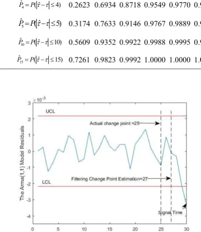
S&P500 index’s real case
As it is shown, the Shewhart control diagram emitted an uncontrolled signal at the 30th sample. In order of estimating the real change point, the estimator could be used by filtering. The estimator presented the 28th sample as the filtering change point estimator’s change point.
9. CONCLUSION
In the present study, MLE is introduced in order of estimating the changes of a stationary nature to the
x
control diagram’s ARMA (1, 1) model with the correlation existing amongx
statistics. Filtering, having been considered a DLM estimation process, was utilized in order of estimating unidentified variables following the change point. The performance assessments were carried out by simulating studies on the model of ARMA (1, 1) with a variedφ
coefficient. Simulation findings demonstrated that the estimators suggested a satisfactory performance in order of estimating the change point. In the meantime, with an increase in the shift size, the estimator’s performance was enhanced. In conclusion, a real instance was presented to manifest the application of the uncontrolled method.10. REFERENCES
1. Safaeipour, A. and Niaki, S.T.A., "Drift change point estimation in multistage processes using mle", International Journal of Reliability, Quality and Safety Engineering, Vol. 22, No. 05, (2015), 1550025.
2. Sturludottir, E., Gunnlaugsdottir, H., Nielsen, O.K. and Stefansson, G., "Detection of a changepoint, a mean-shift accompanied with a trend change, in short time-series with autocorrelation", Communications in Statistics-Simulation and Computation, Vol. 46, No. 7, (2017), 5808-5818.
3. Slama, A. and Saggou, H., "A bayesian analysis of a change in the parameters of autoregressive time series", Communications in Statistics-Simulation and Computation, Vol. 46, No. 9, (2017), 7008-7021.
4. Bodnar, O., "Application of the generalized likelihood ratio test for detecting changes in the mean of multivariate garch processes", Communications in Statistics-Simulation and Computation, Vol. 38, No. 5, (2009), 919-938.
5. Doroudyan, M., Owlia, M.S., Sadeghi, H. and Amiri, A., "Monitoring financial processes with arma-garch model based on shewhart control chart (case study: Tehran stock exchange)",
International Journal of Engineering-Transactions B: Applications, Vol. 30, No. 2, (2017), 270-280.
6. Moghadam, R.P., Shahraki, F. and Sadeghi, J., "Online monitoring for industrial processes quality control using time varying parameter model", International Journal of Engineering-Transactions A: Basics, Vol. 31, No. 4, (2018), 524-532.
7. Keramatpour, M., Niaki, S., Khedmati, M. and Soleymanian, M., "Monitoring and change point estimation of ar (1) autocorrelated polynomial profiles", International Journal of Engineering-Transactions C: Aspects, Vol. 26, No. 9, (2013), 933-942. 8. Vakilian, F., Amiri, A. and Sogandi, F., "Isotonic change point
estimation in the ar (1) autocorrelated simple linear profiles",
International Journal of Engineering-Transactions A: Basics, Vol. 28, No. 7, (2015), 1059-1067.
9. Li, F., Tian, Z. and Qi, P., "Structural change monitoring for random coefficient autoregressive time series", Communications in Statistics-Simulation and Computation, Vol. 44, No. 4, (2015), 996-1009.
10. Chang, S.I., Zhang, Z., Koppel, S., Malmir, B., Kong, X., Tsai, T.-R. and Wang, D., "Retrospective analysis for phase i statistical
process control and process capability study using revised sample entropy", Neural Computing and Applications, (2018), 1-14. 11. Ebadi, M., Shahriari, H., Abdollahzadeh, M. and Bahrini, A.,
"Robust estimation of parameters in multivariate processes", in 2011 IEEE International Conference on Quality and Reliability, IEEE., (2011), 585-589.
12. Nishina, K., "A comparison of control charts from the viewpoint of change‐point estimation", Quality and reliability engineering international, Vol. 8, No. 6, (1992), 537-541.
13. Page, E.S., "Continuous inspection schemes", Biometrika, Vol. 41, No. 1/2, (1954), 100-115.
14. Atashgar, K. and Noorossana, R., "An integrating approach to root cause analysis of a bivariate mean vector with a linear trend disturbance", The International Journal of Advanced Manufacturing Technology, Vol. 52, No. 1-4, (2011), 407-420. 15. Ahmadzadeh, F., "Change point detection with multivariate control charts by artificial neural network", The International Journal of Advanced Manufacturing Technology, Vol. 97, No. 9-12, (2018), 3179-3190.
16. Noorossana, R., Saghaei, A., Paynabar, K. and Abdi, S., "Identifying the period of a step change in high‐yield processes",
Quality and Reliability Engineering International, Vol. 25, No. 7, (2009), 875-883.
17. Pignatiello Jr, J.J. and Samuel, T.R., "Estimation of the change point of a normal process mean in spc applications", Journal of Quality technology, Vol. 33, No. 1, (2001), 82-95.
18. Samuel, T.R., Pignatiello Jr, J.J. and Calvin, J.A., "Identifying the time of a step change with x control charts", Quality Engineering, Vol. 10, No. 3, (1998), 521-527.
19. Samuel, T.R., Pignatiello Jr, J.J. and Calvin, J.A., "Identifying the time of a step change in a normal process variance", Quality Engineering, Vol. 10, No. 3, (1998), 529-538.
20. Daryabari, S.A., Malmir, B. and Amiri, A., "Monitoring bernoulli processes considering measurement errors and learning effect",
Quality and Reliability Engineering International, (2019). 21. Perry, M.B., Pignatiello Jr, J.J. and Simpson, J.R., "Estimating the
change point of the process fraction non‐conforming with a monotonic change disturbance in spc", Quality and Reliability Engineering International, Vol. 23, No. 3, (2007), 327-339. 22. Noorossana, R. and Shadman, A., "Estimating the change point
of a normal process mean with a monotonic change", Quality and Reliability Engineering International, Vol. 25, No. 1, (2009), 79-90.
23. Perry, M.B. and Pignatiello Jr, J.J., "Estimation of the change point of a normal process mean with a linear trend disturbance in spc", Quality Technology & Quantitative Management, Vol. 3, No. 3, (2006), 325-334.
24. Perry, M.B., Pignatiello Jr, J.J. and Simpson, J.R., "Estimating the change point of a poisson rate parameter with a linear trend disturbance", Quality and Reliability Engineering International, Vol. 22, No. 4, (2006), 371-384.
25. Ghazanfari, M., Alaeddini, A., Niaki, S.T.A. and Aryanezhad, M.B., "A clustering approach to identify the time of a step change in shewhart control charts", Quality and Reliability Engineering International, Vol. 24, No. 7, (2008), 765-778.
26. Alaeddini, A., Ghazanfari, M. and Nayeri, M.A., "A hybrid fuzzy-statistical clustering approach for estimating the time of changes in fixed and variable sampling control charts", Information Sciences, Vol. 179, No. 11, (2009), 1769-1784.
27. Amiri, A. and Allahyari, S., "Change point estimation methods for control chart postsignal diagnostics: A literature review",
28. Kazemzadeh, R.B., Noorossana, R. and Ayoubi, M., "Change point estimation of multivariate linear profiles under linear drift",
Communications in Statistics-Simulation and Computation, Vol. 44, No. 6, (2015), 1570-1599.
29. Doǧu, E. and Kocakoç, İ.D., "Estimation of change point in generalized variance control chart", Communications in
Statistics—Simulation and Computation®, Vol. 40, No. 3, (2011), 345-363.
30. Lee, J. and Park, C., "Estimation of the change point in monitoring the process mean and variance", Communications in Statistics— Simulation and Computation®, Vol. 36, No. 6, (2007), 1333-1345.
31. Chang, S.T. and Lu, K.P., "Change‐point detection for shifts in control charts using em change‐point algorithms", Quality and Reliability Engineering International, Vol. 32, No. 3, (2016), 889-900.
32. Asghari Torkamani, E., Niaki, S.T.A., Aminnayeri, M. and Davoodi, M., "Estimating the change point of correlated poisson count processes", Quality Engineering, Vol. 26, No. 2, (2014), 182-195.
33. Ayoubi, M., Kazemzadeh, R., Niaki, S. and Amiri, A., Change point estimation of a multivariate normal process mean using dynamic linear model. 2014, Submitted.
34. Ayoubi, M., Kazemzadeh, R.B. and Noorossana, R., "Change point estimation in the mean of multivariate linear profiles with no change type assumption via dynamic linear model", Quality and Reliability Engineering International, Vol. 32, No. 2, (2016), 403-433.
35. Ayoubi, M., Kazemzadeh, R. and Noorossana, R., "Estimating multivariate linear profiles change point with a monotonic change in the mean of response variables", The International Journal of Advanced Manufacturing Technology, Vol. 75, No. 9-12, (2014), 1537-1556.
36. Sheikhrabori, R., Aminnayeri, M. and Ayoubi, M., "Maximum likelihood estimation of change point from stationary to nonstationary in autoregressive models using dynamic linear model", Quality and Reliability Engineering International, Vol. 34, No. 1, (2018), 27-36.
37. Ashuri, A. and Amiri, A., "Drift change point estimation in autocorrelated poisson count processes using mle approach",
International Journal of Engineering, Vol. 28, No. 7, (2015), 1021-1030.
38. Hawkins, D.M. and Zamba, K., "A change-point model for a shift in variance", Journal of Quality technology, Vol. 37, No. 1, (2005), 21-31.
39. Malela‐Majika, J.C. and Rapoo, E., "Distribution‐free mixed cumulative sum‐exponentially weighted moving average control charts for detecting mean shifts", Quality and Reliability Engineering International, Vol. 33, No. 8, (2017), 1983-2002. 40. Amiri, A. and Zolfaghari, S., "Estimation of change point in
two-stage processes subject to step change and linear trend",
International Journal of Reliability, Quality and Safety Engineering, Vol. 23, No. 02, (2016), 1650007.
41. Daryabari, S.A., Hashemian, S.M., Keyvandarian, A. and Maryam, S.A., "The effects of measurement error on the max ewmams control chart", Communications in Statistics-Theory and Methods, Vol. 46, No. 12, (2017), 5766-5778.
42. Lu, K.-P., Chang, S.-T. and Yang, M.-S., "Change-point detection for shifts in control charts using fuzzy shift change-point algorithms", Computers & Industrial Engineering, Vol. 93, No., (2016), 12-27.
43. Jiang, W., Tsui, K.-L. and Woodall, W.H., "A new spc monitoring method: The arma chart", Technometrics, Vol. 42, No. 4, (2000), 399-410.
44. Tsay, R.S. and Tiao, G.C., "Consistent estimates of autoregressive parameters and extended sample autocorrelation function for stationary and nonstationary arma models", Journal of the American Statistical Association, Vol. 79, No. 385, (1984), 84-96.
45. Shao, Q. and Yang, L., "Oracally efficient estimation and consistent model selection for auto‐regressive moving average time series with trend", Journal of the Royal Statistical Society: Series B (Statistical Methodology), Vol. 79, No. 2, (2017), 507-524.
46. Ghanbarzadeh, M. and Aminghafari, M., "A new hybrid-multiscale ssa prediction of non-stationary time series",
Fluctuation and Noise Letters, Vol. 15, No. 01, (2016), 1650005.
47. Montgomery, D.C., "Introduction to statistical quality control, John Wiley & Sons, (2007).
48. Petris G, Petrone S and P, C., "Dynamic linear models with r. , New York, Springer-Verlag, (2007).
49. Meinhold, R.J. and Singpurwalla, N.D., "Understanding the kalman filter", The American Statistician, Vol. 37, No. 2, (1983), 123-127.
50. Zhang, Y. and Li, X., "Fixed-interval smoothing algorithm based on singular value decomposition", in Control Applications, 1996., Proceedings of the 1996 IEEE International Conference on, IEEE., (1996), 916-921.
51. Wang, L., Libert, G. and Manneback, P., "Kalman filter algorithm based on singular value decomposition", in Decision and Control, 1992., Proceedings of the 31st IEEE Conference on, IEEE., (1992), 1224-1229.
52. Francq, C., Roy, R. and Zakoïan, J.-M., "Diagnostic checking in arma models with uncorrelated errors", Journal of the American Statistical Association, Vol. 100, No. 470, (2005), 532-544.
APPENDIX A:
In ARMA(1,1) we have F =
[
1 0]
[
]
1 21
3 4
1 1 0
0
R R
Q FRF R
R R
′
= = =
[ ]
1 2 1 2 1 2
1
3 4 3 4 1 3 4
1 2
1 2
2 3 2 3
3 4
3 4
1 1
1 1 * *1 0 0
0 0
0
R R R R R R
C R RFQ FR
R R R R R R R
R R R R
RR RR
R R
R R
R R
−
′
= − = −
= − =
−
C is not reversible to use of SVD algorithm. So we couldn’t use of Petris model.
Meinhold and Singpurwalla [49] stated that if X1 and X2
have a bivariate normal distribution with the means µ1 and µ2
, respectively, and a covariance matrix of 11 12
21 22
Σ Σ
Σ Σ
denoted by 1 1 11 12
2 2 21 22
,
X MN X
µ µ
Σ Σ
Σ Σ
, the conditional
distribution of
X
1 givenX
2will be put as follows:1 1
1 2 2 1 12 22 2 2 11 12 22 21
( |X X =x) Nµ +Σ Σ−(x −µ),Σ −Σ Σ Σ−
Let X1 correspond to
1 j j
j
x ψ ε =
θ and X2 correspond to
x
j.Hence,
1 1
1
1 1 1
( | )
( | )
j j j
j
j j j
E D
X
V ar D
−
−
= =
= ⇒ = =
µ θ a
θ
Σ θ R
,
2 j 2 ( j | j 1) j j,
X = x ⇒ µ = E x D − =F a Since Vj=0 in this paper, we have Σ2 2 =V ar x( j |Dj−1)= F R Fj j ′.
Due to the ARMA (1,1) model of
0 1 1 1
j j j j
x
=
φ
x
−+
ε
+
ϕ ε
−and E(ε j)= E(ε j−1) = 0, we can substitute 2
1 1
( j | )
j j j
x
E D
x
ψ ε −
with
2
1 1
2
1 1 1 1 1
2
2 1
var( | D ) ( | D )
[ ( ) | ]
( )
j j j j
j j j j j j j
j j j j j
x E x
Eψ ε φ x ψ ε ε ε D
ψ σ
− −
− − −
+
=
+ +
′
+
F R F F a
Also, it is realized that
1 1
( | )
0
j j j
j j x
E D
ψ ε −
=
F a .
So, 12 2
2 2
1 1
( ) 0
j j
j j
j j j j j
j j ψ σ
ψ σ
=
′ ′
+ − × =
Σ
F R F F a
F R F F a
F a
As a result, the following equation can be obtained according to equation (A1):
1 1 22
1 2
1 2
1
var( | , ) var( | )
*( ) *
j j j j
j j
j j
j j j j j
x D D
ψ σ ψ σ
− −
−
= =
= − =
′
′ ′
−
11 12 21
C θ
θ Σ Σ Σ Σ
F R F
R F R F F R F
1 1 22
1 2
1 2
1
var( | , ) var( | )
*( ) *
j j j j
j j
j j
j j j j j
x D D
ψ σ ψ σ
− −
−
= =
= − =
′
′ ′
−
11 12 21
C θ
θ Σ Σ Σ Σ
F R F
R F R F F R F
Change Point Estimation of the Stationary State in Auto Regressive Moving Average
Models, Using Maximum Likelihood Estimation and Singular Value
Decomposition-based Filtering
R. Sheikhraboria, M. Aminnayeria, M. Ayoubib
a Department of Industrial Engineering and Management Systems, Amirkabir University of Technology, Tehran, Iran bDepartment of Industrial Engineering, College of Engineering, West Tehran Branch, Islamic Azad University, Tehran, Iran
P A P E R I N F O
Paper history:
Received 26 Januray 2019
Received in revised form 06 March 2019 Accepted 07 March 2019
Keywords:
Auto Regressive Moving AverageModel Change Point Estimation
Dynamic Linear Model Maximum Likelihood Estimation Singular Value Decomposition
. ! " # $ % & !
'( $) . ! * + ) , -! ("! .+ ) / (# $ "(+
01 2 ( ( , 4 $) 5 ) 7( "8 2 )- 9 8- : " ,
* ;"! ;(
( *)< $) . ! *)<
%< = " . + ... * % ) > ( 9 ?! @ A : :
!
! *)< 9 ?! ?(B , $) -C + $ . / (A : . ! ?(B , $) + +
.
doi: 10.5829/ije.2019.32.05b.15
12 1 1
1 2
1 1 1
1 1
( , | ) ( , | )
( | ) ( | ) ( | )
j
j j j j j
j
j j
j j j j
j
j j
x
Cov x D Cov x D
x x
E D E D E x D
x
ψ ε
ψ ε ψ ε
− −
− − −
= =
= − ×