A Boundary Meshless Method for Neumann Problem
K. Maleknejad
*and P. Torabi
Department of Applied Mathematics, Faculty of Mathematics, Iran University of Science and Technology, Tehran, Islamic Republic of Iran
Received: 24 October 2010 / Revised: 17 September 2011 / Accepted: 8 November 2011
Abstract
Boundary integral equations (BIE) are reformulations of boundary value
problems for partial differential equations. There is a plethora of research on
numerical methods for all types of these equations such as solving by
discretization which includes numerical integration. In this paper, the Neumann
problem is reformulated to a BIE, and then moving least squares as a meshless
method is described for solving this integral equation. Error analysis of this
method is discussed and then its application and accuracy are illustrated by some
case studies.
Keywords: Laplace’s equation; Neumann problem; Boundary integral equation; Meshless method; Moving least squares method
*
Corresponding author, Tel.: +98(912)1025511, Fax: :+98(21)73225416, E-mail: [email protected] Introduction
Laplace’s equation is a second order partial differential equation as
0 ,
u in D
where is the Laplace operator and u is a scalar function of two or three variables. The general theory of solution to Laplace's equation is known as potential theory. The solutions of Laplace's equation are all harmonic functions which are important in many fields of science, notably the fields of electromagnetism, astronomy and fluid dynamics. The Dirichlet problem for Laplace's equation consists of finding a solution u on some domain D such that u on the boundary of D
satisfies
, ,
u f on S D
where f is a given function. The Neumann boundary conditions for Laplace's equation specify not the function u itself on the boundary of D, but its normal derivative
, .
u
f on S D n
Vol. 22 No. 3 Summer 2011 Maleknejad and Torabi J. Sci. I. R. Iran
For the Dirichlet problem, if a solution exists, it is unique; and for the Neumann problem, it is unique to within an arbitrary constant. The existence theorem, however, is more difficult to prove (see [1]).
There are various numerical methods to solve these problems. One of them is the finite difference method (FDM) for the solution of differential equations, especially, for boundary value problems.
Another numerical technique for finding approxi-mate solutions of partial differential equation is the finite element method (FEM). The solution approach is based either on eliminating the differential equation completely or rendering the partial differential equation into an approximating system of ordering differential equation, which are then numerically integrated using standard techniques such as Euler's method, Runge-Kutta, etc. In solving partial differential equations, the primary challenge is to create an equation that approximates the equation under study, and is also numerically stable. This means that errors in the input and intermediate calculations do not accumulate and, therefore, do not cause the resulting output to be meaningless. In so doing, there are several ways, all of which have both advantages and disadvantages. The Finite Element Method is a good choice for solving partial differential equations over complicated domains (like cars and oil pipelines), when the domain changes (as during a solid state reaction with a moving boundary), when the desired precision varies over the entire domain, or when the solution lacks smoothness. For instance, in a frontal crash simulation it is possible to increase prediction accuracy in important areas like the front of the car and reduce it in its rear. The differences between FEM and FDM are:
The most attractive feature of the FEM is its ability to handle complicated geometries (and boundaries) with relative ease. While FDM in its basic form is restricted to handle rectangular shapes and simple alterations thereof, the handling of geometries in FEM is theoretically straightforward.
The most attractive feature of finite differences is that it can be very easy to implement.
There are several ways one could consider the FDM a special case of the FEM approach. One might choose basis functions as either piecewise constant functions or Dirac delta functions. In both approaches, the approximations are defined on the entire domain, but need not be continuous. Alternatively, one might define the function on a discrete domain, with the result that the continuous differential operator no longer makes sense, however this approach is not FEM.
There are reasons to consider the mathematical
foundation of the finite element approximation more sound, for instance, because the quality of the approximation between grid points is poor in FDM. The quality of a FEM approximation is often higher
than in the corresponding FDM approach, but this extremely depend on problem and several examples to the contrary can be provided.
The finite volume method (FVM) is a method for representing and evaluating partial differential equations in the form of algebraic equations (see [2]). Similar to the finite difference method or finite element method, values are calculated at discrete places on a meshed geometry. "Finite volume" refers to the small volume surrounding each node point on a mesh. In the finite volume method, volume integrals in a partial differential equation that contain a divergence term are converted to surface integrals. These integrals are then evaluated as fluxes at the surfaces of each finite volume. Because the flux entering a given volume is identical to that leaving the adjacent volume, these methods are conservative. Another advantage of the finite volume method is that it is easily formulated to allow for unstructured meshes.
B
In this equation to s an important purpose, we Let D be a bo plane, and le with a param ( )t ( ( r
with rC2
assume the p clockwise di normal n( )t
( ( )t
n The Neu 1 ( )
uC D
( ) ( ) u P u P f P n
with f C
following th the solution.
Theorem 1. parameteriza
Neumann pr addition of an
( ) Sf Q dS
A very im differential Gauss's theor
Theorem 2. of F containe
. ( D Q
FUsing th Green's iden Assuming u
Green's first
Boundary In
section, we solve the Neum t kind of boun
use the notati ounded open s et its boundar meterization
( ), ( )), 0t t
[0, ]L and | parameterizat irection and th
that is orthog
2 2 ( ), ( )) ( ) ( ) t t t t umann prob 2 ( ) C D
that
0, ,
( ),
P D
f P P S
( )
C S a give
eorem in [6]
. Let the fun ation of (1), a
roblem has a n arbitrary con
0.
S
mportant too equations is rem.
Assume F:D
ed in C D1( ).
) (
S
dD
FQhe divergence ntities and Gr
1
( )
C D
and
identity by let
ntegral Met
employ bo mann problem ndary value pr on which has simply connec ry S be a sim
, t L
( ) | 0t
r for
tion traverses hen introduce gonal to the cu
.
blem is as satisfies
,
en boundary
guarantees th
nction f C(
ssume rC2
a unique solu nstant, provid
l for studyin the diverge
2
DR with Then
). ( ) .
Q nQ dS
e theorem, reen's represe d vC2( )D
tting F u v thod
oundary integ m which in tur
roblems. For been used in cted region in mple closed cu
r 0 t L. S in a coun e the interior u urve S at ( )rt
follows: F
function. T
he uniqueness
( )S , and for
2
[0, ]L . Then ution, up to ded
g elliptic par nce theorem
each compon
one can obt entation formu
, one can pr
v in (3)
gral rn is this [6]. n the urve (1) We nter-unit : Find The s of the the the (2) rtial or nent (3) tain mula. rove of one Ne the Ne con for fun a w ref to be def wh of
Du vdD
Next, assume
u and v in (4) e may obtain
[
D u v v
The identity eumann proble e addition of eumann probl ndition (2) is n
Another tool r Laplace’s ndamental sol weighting fun formulation of introduce Dir a sequence fined as below
2 ( ) 0 n n w x
hich shown in Then we def the sequence
( ) lim n
x w
Figure 1. I . D u vdD
e u v, C2(D
) and then sub Green's secon
] [
S
u dD v
(4) can be em has a solut f an arbitrary
lem is to ha necessary. l that we nee
equation i ution of a par nction that is f the equation rac delta func
of unit forc w 1 | | , 1 | | x n x n Figure 1. fine the Dirac
( ). n
w x
Illustrations of u S
v u dS
n)
D . Interchang btracting the t nd identity
]
u v
u dS
n n
used to pro tion, then it is y constant; an have a soluti
ed is fundame in two var rtial differenti
used to boun n. For this purp ction. Suppos
ce distribution
,
delta functio
unit force distri
. (4)
ging the roles
two identities,
.
S (5)
ove (i) if the s unique up to nd (ii) if the on, then the
ental solution riables. The ial equation is ndary integral pose, we have e {wn( )}x n1
ns which are
on as the limit
Vol. 22 No. 3 Summer 2011 Maleknejad and Torabi J. Sci. I. R. Iran
The Dirac delta function is not a function in the usual sense, because we have ( )x 0 for x 0 and
(0)
, it is, therefore, more correctly referred to as the Dirac delta distribution. It has properties which are mentioned below
a) We have ( )x dx 1
since wn( )x dx 1
for all n1.b) For any continuous function h x( ): ( ) ( )x h x dx h(0).
c) In general, for any constant : ( x h x dx) ( ) h( ).
d) The Dirac delta function is the slope of the Heaviside step function
0
( )
1
if x
H x
if x
(where is a constant): ( x)H(x).
Laplace’s equation, as well as most of the common equations, has a well-known fundamental solution. The fundamental solution is a solution of the following equation for an arbitrary point AD
( ) 0,
w A Q
It means w is a solution of w 0 which has a singularity at the point A. This is not difficult to find this solution, and one can see [7] for a description of the manner in which w can be determined. In 2-D Laplace’s equation the fundamental solution is
1
w(Q) log|A Q|
2
.
Assume uC2(D), where u(Q) be a solution of Laplace's equation, and let v(Q)log|A Q| , with
AD. Since ( ) 1 ( ) 2
w Q v Q
and w(Q) is the fundamental solution, then
1
( ) 0, 2 v A Q
or
2 ( ).
v A Q
Also we have u 0, because we supposed that u(Q) be a solution of Laplace’s equation. Now by replacing them into the Green’s second identity (5) we will have the following relation
( )
2 ( ) [ log | |
( )
( ) [log | |]] , ,
( ) S
Q u Q
u A A Q
Q
u Q A Q dS A D
Q
nn
(6)
where the property (c) of Dirac delta function is used in the left side. Assume PS , and A tends to P, then we obtain the following limits where one can find a proof of them in [8] or other text on Laplace’s equation
( )
lim log | |
( )
( )
log | | ,
( ) Q S
A P
Q S
u Q
A Q dS Q
u Q
P Q dS Q
nn
and
lim ( ) [log | |]
( )
( ) ( ) [log | |]
( ) .
Q S
A P
Q S
u Q A Q dS
Q
u P u Q P Q dS
Q
nn
By taking limit for both side of the equation (6) and using the above relations we have
1 ( )
( ) [ log | |
( )
( ) [log | |]] , ,
( ) S
Q u Q
u P P Q
Q
u Q P Q dS P S
Q
nn
(7)
which gives a relationship between the values of u and its normal derivative on S. By using the boundary condition of the Neumann problem, u n f on S, we rewrite (7) as follows
1
( ) ( ) [log | |]
( )
1
( ) log | | , .
Q S
Q S
u P u Q P Q dS
Q
f Q P Q dS P S
n(8)
The equation (8) is an integral equation of the second kind which is solvable if and only if the boundary function f satisfies the condition (2). Unfortunately, it is not uniquely solvable. The simplest way to deal with the lack of uniqueness in solving (8) is to introduce an additional condition such as
*
( ) 0, u P
for some fixed point P*S . Let u (Q)1 and u (Q)2 be
above condition. By choosing PP* and uu1 or 2
u , the equation (8) implies
* 1
*
( ) [log | |] ( )
( ) log | | , Q
S
Q S
u Q P Q dS Q
f Q P Q dS
n
* 2
*
( ) [log | |] ( )
( ) log | | , Q
S
Q S
u Q P Q dS Q
f Q P Q dS
n
which in turn imply u (Q)=u (Q)1 2 . Thus the equation (8) has a unique solution. When the representation
( )t ( ( ), ( )) t t
r of (1) for S is applied to integral equation (8), this equation becomes
0
( ) L ( , ) ( ) ( ), 0 ,
u t K t s u s ds g t t L
(9)with
2 2
( )[ ( ) ( )] ( )[ ( ) ( )]
( , ) , ,
[ ( ) ( )] [ ( ) ( )]
s t s s t s
K t s s t
t s t s
2 2
( ) ( ) ( ) ( )
( , ) ,
2[ ( ) ( ) ]
t t t t
K t t
t t
and the right hand side
2 2
0
( ) L ( ( )) ( ) ( ) log | ( ) ( ) | .
g t
f rs t t rt r s dsThe solution of this Fredholm integral equation of the second kind is the solution of the Neumann problem on the boundary of D. Let 1
( )
u C D
i i be a solution
of Laplace's equation in Di (interior of D), then ui satisfies the following relation (see [6])
( ) ( ) [log | |] , ,
( ) Q i
S
u A u Q A Q dS A D
i Q
nwith using (1) for S it takes the form
0
( , ) L ( , , ) ( ) , ( , ) ,
i i
u x y
M x y s u s ds x y D (10)2 2
( )[ ( ) ] ( )[ ( ) ]
( , , ) .
[ ( ) ] [ ( ) ]
s s x s s y
M x y s
s x s y
Fredholm integral equation (9) can be solved with any methods which have been described in books on integral equations. In this paper, we solve it by a meshless method which is based on the moving least square (MLS) method (see [9]). This method does not
require any background interpolation or approximation cells and does not depend on the geometry of domain. It is, therefore, suitable for problems with any kind of domains.
Moving Least Squares Method
For a better sense of moving least squares (MLS), we introduce least squares (LS) and weighted least square (WLS) at first. Given n points where located at positions
d i
x R for i 1,...,n. We wish to obtain a globally defined function uh( )x
that approximates the given scalar values ui at points xi in the least-squares sense with the error functional h( ) 2
i
LS i i
J ‖u x u ‖ . Thus, we pose the following minimization problem
2
min h( ) ,
i h d
m i i
u
u x
u‖
‖
(11)where h
u is taken from dm, the space of polynomials of total degree m in d spatial dimensions, and it can be written as
( ) ( ) ( ). ,
h T
u x p x a p x a (12)
where p x( )[p1( ),...,x pk( )]x T is the polynomial basis vector and [ ,...,1 ]
T k
a a
a is the vector of unknown coefficients, which we want to minimize in (11). We can minimize (11) by setting the partial derivatives of the error functional JLS to zero, i.e. JLS 0, where
1
[ / ,..., / ]T k
a a
, which is a necessary condition for a minimization. Then we obtain a linear system of equations
( ) ( )T ( ) ,
i i i i
i i
u
p x p x a p x
which is solved as
1
[ ( i) ( i)T] ( i) i.
i i
u
a p x p x p x (13)
If the square matrix ( ) ( )T i
LS i i
A p x p x is nonsingular, replacing Eq. (13) into Eq. (12) provides the fit function uh( )x .
In the weighted least squares formulation, for a fixed point x R d, we minimize
2
min ( ) ( ) .
h d m
h
i i i
u i
w u u
‖x x ‖‖ x ‖ (14)Vol. 22 No. 3 Summer 2011 Maleknejad and Torabi J. Sci. I. R. Iran
least squares approximation in x is written as ( ) ( ) ( ) ( ). ( ).
h T
ux x p x a x p x a x (15)
By taking partial derivatives of the error functional W LS
J with respect to the unknown coefficients ( )a x we obtain
1
( ) [ ( ) ( ) ( ) ]
. ( ) ( ) .
T
i i i
i
i i i i
w
w u
a x x x p x p x
x x p x
‖ ‖
‖ ‖
(16)
Obviously, the only difference between Eqs. (13) and (16) is the weighting terms. Note that whereas the coefficients a in Eq. (13) are global, the coefficients
( )
a x are local and need to be recomputed for every x. If the square matrix AWLS iw(‖x x i ‖) (p x p xi) ( i)T is nonsingular, replacing Eq. (16) into Eq. (15) provides the fit function h( )
ux x .
The MLS method was proposed by Lancaster and Salkauskas [5] for smoothing and interpolating data. The idea is to start with a weighted least squares formulation for an arbitrary fixed point in Rd, and then move this point over the entire parameter domain, where a weighted least squares fit is computed and evaluated for each point individually. It can be shown that the global function uh( )x , obtained from a set of local functions,
( ) ( ),
h h
u x ux x
2
,
min ( ) ( )
h d m
h
i i i
u i
w u u
x x
x x x
‖ ‖‖ ‖
is continuously differentiable if and only if the weighting function is continuously differentiable (see Levins work [10,11]).
Now we extend the MLS method for BIE which is obtained in the previous section. For this purpose, we follow [9]. Given data values { } 1
N j j
u
u at nodes xj , the MLS method produces a function uhCs(Rd) that approximates data u in a weighted square sense. Let
d q
be the space of polynomials of degree q, qN
and qs , and let {p0,p1,...,pm} be any basis of d q
.
The MLS approximation uh( )x of u( )x for all x, can be defined as
( ) ( ), ,
h T
u x P a x x (17)
where ( ) [ 0, 1,..., ]
T
m
p p p
P x and a x( ) is a vector with
components a ( )j x , j 0,1,...,m, which are functions of the space coordinates x. In this paper we suppose that the basis of dq is a complete monomial basis of order m .For example, for a 1-D problem, the linear basis is {1, }x , and the quadratic basis is {1, ,x x2}
. For a 2-D problem, the linear basis is {1, , }x y , and the quadratic basis is 2 2
{1, , ,x y x ,xy y, } where x( , )x y . The coefficient vector a x( ) is determined by minimizing a weight discrete square norm, which is defined as (u is a scalar function)
2
1
( ) ( )( ( ) ( ) )
[ . ( ) ] . .[ . ( ) ], n
T
j j j
j
T
J w P u
P W P
x x x a x
a x u a x u
(18)
where w ( )j x is the weight function associated with the
node j and n is the number of nodes in for which the weight function w ( )j x 0 and uj are the fictitious nodal values, but not the nodal values of the unknown trial function h( )
u x i.e. h( ) j j
u x u . The matrices P
and W are defined as
1
1 2
( 1)
( )
( ) 0
( )
, .
0 ( )
( ) T T
n
T n n
n n m
w
P W
w
p x
x p x
x p x
The stationary point of J, in Eq. (18), with respect to ( )
a x leads to the following linear relation between ( )
a x and u
( ) ( ) ( ) ,
A x a x B x u (19)
where the matrices A( )x and B( )x are defined by
1
( ) ( ) ( ) ( ) ( ),
n
T T
j j j
j
A P W P B P w x
x x p x p x
1 1 2 2
( )
[ ( ) ( ), ( ) ( ),..., ( ) ( )]. T
n n
B P W
w w w
x
x p x x p x x p x
The matrix A is often called the moment matrix, it is of size (m 1) (m 1) . Computing a x( ), using Eq. (19) and substituting it into Eq. (17), gives
1
( ) ( ). ( ) , ,
n
h T
j j j
u u
x x u x x (20)
1
( ) ( ) ( ) ( ),
T T
A B
x p x x x
or
0
1
( ) ( )[ ( ) ( )] . m
j k
k
p A B kj
x x x x (21)
( ) j
x ’s are called the shape functions of the MLS approximation, corresponding to nodal points xj . Remark 3. In Eq. (21), to avoid calculating A1, we can get C A B1 and then solve the systems A C B and since for j( )x , only components of j-th column of
C are needed, it is enough to solve only linear system j j
AC B which Cj and Bj are j-th column of C and
B, respectively. This system can be solved by iterative methods.
If wj( )x Cr( ) and ( ) ( ) s k
p x C , j 1, , n, k0,1,, m then j( )x Cmin r s( , )( ) . The Gaussian weight function is applied in the present work as
2 2
2
w (x)=
0,
[ ( / ) ] [ ( / ) ]
, 0 ,
d >h ,
1 [ ( / ) ]
j
j j
j j
j j j
exp d exp h
d h exp h
where dj x x j (the Euclidean distance between x and xj), is a constant which controls the shape of the weight function w , and j h is the size of the j
support domain.
Integral Equation and MLS
In this section, we follow [9] to solve an integral equation by MLS method. Then we use it for BIE which has been obtained in section 2. Consider Fredholm integral equation
( ) b ( , ) ( ) ( ), [ , ],
a
u x x u d g x x a b
(22)where u is unknown function, is a real parameter, a
and b are finite real numbers and (x, ) is called kernel function. Assume that u, , and g have necessary conditions for solvability of the equation and analyzing the method.
To apply the method, at first N nodal points {x }i are
selected on interval [ , ]a b where ax1x2...
N
x b
. The distribution of nodes could be selected regularly or randomly. Then we can use h
u from Eq.
(20) instead of u. So Eq. (22) becomes
( ) b ( , ) ( ) ( ), [ , ],
h h
a
u x x u d g x x a b
(23)or equivalently
1
[ ( ) ( , ) ( ) ] ( ), [ , ],
N b
j a j j
j
x x d u g x x a b
Assume that the above Eq. holds at xi
1
[ ( ) ( , ) ( ) ]
i=1,2,...N
( ), .
N b
j i a i j j
j
i
x x d u
g x
(24)
Using a m1-point quadrature formula with the
coefficients {k} and weights {k} in interval [ , ]a b to
numerically solve the integration in (24), yielding
1
1 1
ˆ
[ ( ) ( , ) ( )
i=1,2,...N
]
( ), .
m N
j i i k j k k j
j k
i
x x u
g x
(25)
where uˆj are the approximate values of uj when we use a quadrature rule instead of the exact integral. Now if we set F as an N by N matrix which is defined by
1
,
1
( ) ( , ) ( ) ,
m
i j j i i k j k k k
F x x d
and vectors
1 2
ˆ ˆ ˆ
[ ,u u ,...,uN] ,T
u
and
1 2
[ , ,..., ] ,T N
g g g
g
then we have the following linear system of equations .
Fu g (26)
By solving Eq. (26) with a proper numerical method such as Gauss elimination method or LU factorization, we find values of uˆj . Then the value of u(x) at any point x[ , ]a b can be approximated by Eq. (20) as
1
ˆ
( ) ( ) ( ) , [ , ].
n
N j j
j
u x u x x u x a b
Vol. 22 No. 3 Summer 2011 Maleknejad and Torabi J. Sci. I. R. Iran
Error Analysis
The error analysis of this method is based on what has been described in [9]. We write Eq. (22) in operator form as
()u g, (27)
where
( , ) ( ) . b
a
u
x u d
Similarly Eq. (23) can be written as
()uh g, (28)
and assume that is a compact operator (for more details about the compact integral operators see chapter 1 of [6]). From [9] we have the following lemma and theorems.
Theorem 4. There exist constants Cr, r1, 2, such that for each r,1( )
uC
1 | | ,1
( ) ,0 | | .
h r
r r
L
D u D u C R u r
∣ ∣
where Ris an upper bound of the mesh-size.
Lemma 5. If (27) be uniquely solvable and 0
h uu
then (28) is uniquely solvable.
The approximation scheme for numerical integration can be written as
(M)uN g.
Now the following theorem shows the convergence analysis of the method in L norm.
Theorem 6. Let uCr,1( )( r1, 2) where be a closed, bounded set in Rd and let (x, ) be continuous for ,x . Assume the quadrature sche-me is convergent for all continuous functions on . Further, assume that the integral equation (27) is uniquely solvable for given gC( ) with 0. Moreover take a suitable approximation h
u of u. Then for all sufficiently large values of M , the approximate inverses
1
( M)
exist and are uniformly bounded,
1 1
1
1 ( ) .
( )
( ) . ( )
,
M M
M M M
Q
∣ ∣
with a suitable constant Q . For the equations
()u g and (M)uN g, we have
1 ,1
( ) ( )
( ) ( )
(1 )
, r
N L r r M L
M L L
u u C R u Q F F
Q F F u
∣ ∣
where R and Cr are introduced in Theorem 4. Let (N)( , )
i
u x y be the solution of (10) by using the approximation solution uN
( )
0
( , ) L ( , , ) ( ) , N
i N
u x y
M x y s u s ds (29) and let (N m, )i
u denote the result of approximation
( )
( , ) N i
u x y using a quadrature rule
( )
1
( , ) ( , , ) ( ).
m N
i j j N j
j
u x y w M x y x u x
Such as [6], for a convex region
( ) ( , )
max ( , ) ( , ) 2 .
i
N
i i N L
x y D
u x y u x y u u
∣ ∣
The total error is given by
( , ) ( )
( ) ( , )
( , ) ( , ) [ ( , ) ( , )] [ ( , ) ( , )].
N m N
i i i
N N m
i i
u x y u x y u x y u x y i
u x y u x y
Results and Discussion
In this section, efficiency and accuracy of the method are illustrated by some numerical examples. The routines are written in Fortran 90.
Example 1. This example is solved in [6] as a Dirichlet problem and we solve it as a Neumann problem with our proposed method. Let the boundary S be the ellipse
cos , sin
, 0 2 . r t a t b t t In this case, the kernel K of (9) can be reduced to
( , ) ( ),
2 s t K t s
2 2 2 2
( ) ,
2[ ( ) ( )]
ab
a sin b cos
and the integral equation (9) becomes
2
0
( ) ( ) ( ) ( ), 0 2 .
2 s t
u t u s ds g t t
Table 1, indicates the results of solving this equation with
cos
( , ) x y,( , ) .
f x y e x y S
The exact solution u is not known explicitly; but we obtain a highly accurate solution by using a large value of N , and then this solution is used to calculate the errors shown in the table. Results are given for
( , )a b (1, 5). We put 1 (N 1) then for the linear case hj 2 and for the quadratic case hj 2.5 to ensure the regularity of moment matrix A in MLS approximation. Besides, 0.6 in both cases. Because of increasing the condition number of A, the error increases in quadratic case as Table 1 shows (see [12]). To evaluate (N)( , )
i
u x y from Eq. (29), we use the trapezoidal rule and as shown in Table 1, we choose
mN. The error along the line
( ) ( cos , 0 1,
4
q q a q c
is shown in Table 2.
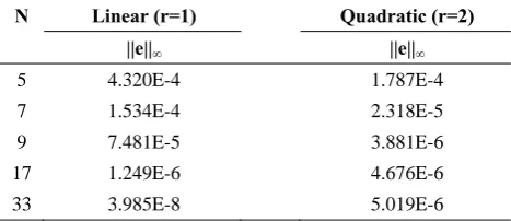
Example 2. Consider the boundary S be the circle ( ) (cos(2 ), sin(2 )), 0 1,
r t t t t
and boundary condition with ( ) cos(2 ).
f t t
The unique exact solution of this problem is
( ) (2 ).
u t cos t
Errors of the approximation solution are given in Table 3, and (N m, )
i i
u u along the line
( ) ( cos , sin ), 0 1,
4 4
q q a b q c
is shown in Table 4.
According to these numerical experiments, the obtained errors and the advantages mentioned in the previous sections guarantee the efficiency and trustworthy of the proposed method.
In this paper, we used the property of boundary integral equation to reduce the 2-D Neumann problem to an integral equation in one dimensional space. In addition, we utilize MLS as a meshless method for solving arisen integral equation. Since this method does not need to take a mesh in domain and only requires some scattering nodes, it is very useful for problems in
high dimensions. One can easily extend this method to three dimensional Neumann problem and Dirichlet problem.
Table 1.MaximumerrorsfordifferentvaluesofNinexample1 N Linear (r=1) Quadratic (r=2)
||e||∞ ||e||∞
5 2.945E-3 2.184E-5 7 1.383E-3 2.484E-4 9 6.852E-4 1.215E-5
17 9.926E-5 7.326E-4
33 1.011E-7 3.629E-4
Table 2. Error ui(c(q))u( N,m)i ( (q))c for some q in example 1
q m=7 m=9 m=17 m=33 0.0 3.623E-1 2.071E-2 2.071E-3 3.671E-4 0.2 3.031E-1 2.165E-2 8.701E-4 3.235E-5 0.4 2.573E-2 8.763E-3 3.763E-4 2.238E-5 0.6 1.150E-2 5.132E-4 1.670E-4 4.060E-6 0.8 1.335E-3 6.411E-4 2.495E-5 3.101E-6 0.9 3.592E-2 5.739E-3 3.145E-3 2.056E-5
Table 3.MaximumerrorsfordifferentvaluesofNinexample2 N Linear (r=1) Quadratic (r=2)
||e||∞ ||e||∞
5 4.320E-4 1.787E-4 7 1.534E-4 2.318E-5 9 7.481E-5 3.881E-6
17 1.249E-6 4.676E-6
33 3.985E-8 5.019E-6
Table 4. Error ui(c(q))u( N,m)i ( (q))c for some q in example 2
q m=7 m=9 m=17 m=33
Vol. 22 No. 3 Summer 2011 Maleknejad and Torabi J. Sci. I. R. Iran
References
1. Kellogg D., Foundation of Potential Theory, Dover, (1953).
2. LeVeque, Randall, Finite Volume Methods for Hyperbolic Problems, Cambridge University Press (2002).
3. Maleknejad K., Mesgarani H., Numerical method for a nonlinear boundary integral equation, Applied Mathematics and computation 182: 1006-1009 (2006). 4. Shepard D., A two dimensional interpolation function for
irregularly spaced points, in: Proc. 23rd Nat.Conf. ACM, ACM Press, New York (1968).
5. Lancaster P., Salkauskas K., Surfaces generated by moving least squares methods, Math. Comput. 37: 141-158 (1981).
6. Atkinson K.E., The Numerical Solution of Integral Equations of the Second Kind, Cambridge University Press, New York (1997).
7. Liu Y., Fast Multipole Boundary Element Method, Theory and Application in Engineering, Cambridge University Press (2009).
8. Colton D., Partial Differential Equations: An Introduction, Random House, New York (1988).
9. Mirzaei D., Dehghan M., A meshless based method for solution of integral equations, Applied Numerical Mathematics 60: 245-262 (2010).
10. Levin D., The approximation power of moving least-squares, Math. Comp., 67(224): 1517-1531 (1998). 11. Levin D., Mesh-independent surface interpolation, to
appear in ’geometric modeling for scientific visualization’ edited by brunnett, hamann and mueller, springer-verlag (2003).