Please cite this article as: M. Nouri Koupaei, M. Mohammadi, B. Naderi,Optimizing Flexible Manufacturing System: A Developed Computer Simulation Model, International Journal of Engineering (IJE), TRANSACTIONS B: Applications Vol. 29, No. 8, (August 2016) 1112-1119
International Journal of Engineering
J o u r n a l H o m e p a g e : w w w . i j e . i rOptimizing Flexible Manufacturing System: A Developed Computer Simulation
Model
M. Nouri Koupaei, M. Mohammadi*, B. Naderi
Department of Industrial Engineering, Faculty of Engineering, Kharazmi University, Tehran, Iran
P A P E R I N F O
Paper history: Received 21 March 2016
Received in revised form 23 April 2016 Accepted 02 June 2016
Keywords:
Flexible Manufacturing System Computer Simulation Modeling
Traffic Forecasting
A B S T R A C T
In recent years, flexible manufacturing system as a response to market demands has been proposed to increase product diversity, optimum utilization of machines andperiods of short-term products.The development of computer systems has provided the ability to build machines with high functionality and the necessary flexibility to perform various operations. However, due to the complexity and the random nature of these problems, deterministic algorithms are not highly accurate andefficient enough. In this paper, computer simulation models are used to optimize flexible manufacturing system FMS). The objectives of this paper are included:the optimal time served in each unit, the optimal number of servers in each unit, and the optimum number of domestic transportation fleet based on type. At the first step, source-destination traffic matrix is presented for development, including: service time and traffic volume are used. The computational results show the accuracy and efficiency of using simulation tools in these problems.
doi: 10.5829/idosi.ije.2016.29.08b.11
1. INTRODUCTION1
Computer simulation is one of the most powerful tools for process design and analysis of complex systems. Computer simulation is described as a comprehensive method for studying manufacturing systems [1, 2]. In the past, this method rarely used because the low level of computer technology and time-consuming simulation modeling. However, due to the complexity and the random nature these problems, deterministic algorithms are not enough accuracy and efficiency to evaluating [3, 4].
Nowadays, with the increasing ability of computers and specialized software to simulate production, the modeling of complex systems in a relatively short time provided. In other word, todays computer simulations are one of the least costly and best practices in the design of industrial systems has become. Despite the widespread use of simulation, this utility has been less attention on production systems. In the present study, the use of simulation analysis of flexible manufacturing
1*Corresponding Author’s Email: [email protected] (M.
Mohammadi)
system has been studied. With review of literature, this issue will be determined that examining computer simulation of flexible manufacturing system is new and significant issue will be a cornerstone for future research (see Table 1).
production line. On the basis of the predefined requirements of the user, several simulation experiments are suggested [8].
Visuwan and Phruksaphanrat developed a computer simulation of electronic manufacturing service plant [9]. Azadeh et al. integrated modeling of supply chain and information system through a unique integrated meta-heuristic computer simulation algorithm. This research has simulated an actual case study with simulation and in the other stages, has moved forward to improve and optimize the objectives by focusing on a selection of suppliers [10]. Oleskow-Szlapka and Stachowiak use of computer simulation in warehouse automation. The main aim of this research was to automate the warehouse operation as much as possible and to decrease the number of staff in the store. The process was modeled using software FlexSim Simulation Software [11]. Kermanpur et al. presented the solidification process was simulated in both etmacroscopic and microscopic scales [12].
Gao presented a computer simulation of a flexible polymer chain [13]. For some researches, we can refer Zahraee et al. [14], Das et al. [15], Mukherjee and Zohdi [16], Klos and Trebuna [6].
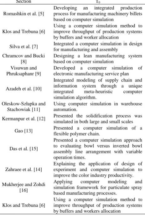
TABLE 1. Literature review based on the aim of papers
Section T0
Romashkin et al. [5]
Developing an integrated production process for manufacturing machinery billets based on computer simulation
Klos and Trebuna [6]
Using a computer simulation method to improve throughput of production systems by buffers and worker allocation
Silva et al. [7] Integrated a computer simulation in design for manufacturing and assembly
Chramcov and Bucki [8]
Designing a lean manufacturing system based on computer simulation
Visuwan and Phruksaphanr [9]
Developed a computer simulation of electronic manufacturing service plan
Azadeh et al. [10]
Integrated modeling of supply chain and information system through a unique integrated meta-heuristic computer simulation algorithm.
Oleskow-Szłapka and Stachowiak [11]
Using computer simulation in warehouse automation.
Kermanpur et al. [12] Presented the solidification process was simulated in both large and small scales
Gao [13] Presented a computer simulation of a flexible polymer chain.
Das et al. [15]
Presented a computer simulation approach to evaluating bowl versus inverted bowl assembly line arrangement with variable operation times.
Zahraee et al. [14]
Explaining the application of design of experiment and computer simulation to improve the color industry productivity.
Mukherjee and Zohdi [16]
Applying computer modeling and simulation framework for particulate spray based manufacturing processes.
Klos and Trebuna [6]
Using a computer simulation method to improve throughput of production systems by buffers and workers allocation
2. SIMULATION MODEL
Computer modeling process are presented in Figure 1. Two main parts of this process is presented in the form of real-world and simulated world. “System Theories” are the representatives of characteristics and system behavior. “System Data” will be collected by “Experiments” on the system. “System Theories” will be determined by “Abstraction” of observations made in the system and “Experiment” is based on data collected. If an initial simulation model of the system is created, “Model Results” can be used in “Hypothesis”. “Validation of System Theories” means a comparison between system theories with system data, to check the accuracy of the system. “Data Collection”,” Abstraction” and “Hypothesis”, will continue to make an acceptable theory of the system.
In the real world there are four basic steps: the actual system goals, system problem, system data and system theories. But in the simulation world there are six basic steps: the simulation model goals, coceptual model, characteristics of simulation models, simulation model, the results of the simulation model and system theories (see Figure 1).
Simulation model made based on a set of predetermined goals. “Conceptual model” is one or more mathematical relations, logic or description that used to describe the goals of a research study and specifically defined.
“Characteristics of Simulation Model” are the full written description of design and software characteristics that is used to convert the conceptual model to computer models. “Simulation model” is actually a computer version of the conceptual model that can be multiple "tested" and “simulation model results” to be recorded.
Conceptual model is prepared with the precise understanding of the system and theoretical modeling. Simulation model is created by using special software and converting the characteristics of the conceptual model to an application language.
“Conceptual model validation” means to compare its characteristics with system theories. In order to ensure proper application used to display the model, an evaluation criterion is done.
Also, “Assessment Modeling” is done to make sure compliance conceptual model with the computer model. Finally, "validation of results" is done to determine the accuracy of the data.
2. 1. Conceptual Model of Flexible Manufacturing
System (FMS) The case study of this paper is one
of the steel companies in Iran. In this company, Entry permit and unloading is given in the trailer carrying the raw material after weighing in the weighing station located at the entrance. For each type of raw material, a certain warehouse is considered. Depending on the load, trailer moves toward the first load from predetermined paths. Accumulation, storage, iron removal and limestone sections are crowded parts of the company. After unloading by trailers, manufacturing sector load again weighed to calculate the net weight. Given that
the system is centralized and automated, so a suitable database have been registered such as: date and time of log trailer to the company, the date and time of leaving the company, tonnage, type of cargo and trailer departed.
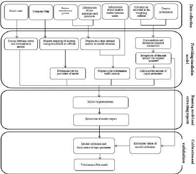
Empty trucks that refer to product loading will follow a similar pattern. First, empty trailer is weighed. According to the type of bill, the trailer being driven to loading blooms, billets or slabs. When leaving the company, trailer again is weighed to calculate the net weight. Trucks will not be distributed at the same time. In other words, entry and exit of trucks will be done in different shifts. According to surveys, 60% of the entry and exit of the factory in the morning shift, 30% in the evening shift and 10% is done in the night shift with the exception of waste transport that can be done only in the morning. In Figure 2, the process of collecting information and conducting simulation of model is provided.
Presence distributing of trailer at a company based on the type of load.
Volume interfering of trailer at intersection.
Figure 2. Modeling process of flexible manufacturing system in case study
vali
d
at
io
The required information about modeling was extracted as follows:
Determining distribution time between truck arrivals to company, based on the type of load.
Determining distribution of service time weighing station.
Determining trailers path between any two company units.
Determining distributions function of accumulation, storage, iron removal, steel material storage, refractory materials warehouse, pelletizing warehouse and general store duration.
Determining distribution function for loading time of Bloom storage units, billets storage and slabs warehouse.
Determining source-destination traffic matrix of the company, based on tonnage displacement and the number of trailers.
Determining distribution downtime and repairs per unit.
The trailer speed on each network.
2. 2. Implementation of the Model and the
Results of Case Study In this study, in order to
facilitate data analysis, we communicatedall the desired output was recorded in real-time on their own tables by Show Flow and MATLAB. Then, the necessarydata were extracted from the model usingstatistical analysis. Implementation of the simulation model above is done in 5 steps:
1.Study and understanding of systems: In the first
stage, the analyst may have a complete understanding of the system performance, including the number, location, performance and relationships, workstations, storage, and material flow achieved.
2.Determine the level simulation: At this stage, the
detailed simulation was determined to prevent of increasing the volume of calculations and prolonged intervention.
3.Data collection and data: To run a simulation
model, needed information and data prepared as distributed statistical. The experimental data were usually raw values and then processed to the statistical distribution.
4. Construction of the base model: After following the above steps, the base model of the system was designed and constructed. The results from implementing this model was matched with the model of a real system. Also, any contrary information was correct. In model creation, some factors affecting the system performance, including inputs and outputs, type of operation (processing) performed by each processor and the relationship between the various components of the system were considered. In the
Figure 3, an example of input data window into the application is shown.
5.Analysis and method selection: At this stage, any
possible changes, before applying the actual system, implemented on the model and the results are compared and evaluated. According to the results of the simulation, the best method for the selected system and in real systems, have been applied.
In the implementation of this model, independent run method has been used. This model has run, 5 times and each time for 3 hours.
Outputs criteria of simulation model include:
Average and largest traffic volume of each arc per hour
Trailers queue length distribution per unit of company
Waiting time distribution of trailers in the queue per unit of company
Volume traffic on the axes intersecting with rail network
Productivity of each server-based on the ratio of operating time to downtime
3. CALIBRATION AND VALIDATION
After modeling software and allocation limits of the system, all model parameters must be determined so that the last performance model is reality. In other words, its purpose is to show appropriate of model with facts available. This process is calibration. In statistics, regression validation is the process of deciding whether the numerical results quantifying hypothesized relationships between variables, obtained from regression analysis, are acceptable as descriptions of the data.
Recent researches in early years show that following calibration and validation techniques are used:
1. Animation: using graphics capabilities of new software, we can study over time the model changes. 2. Comprising with other models: comparison of model results with the results of other prestigious models. 3. Degeneracy test: Studying the behavior of model with determining specific values for the input variables. 4. The validity of events: comparing events with the real system events.
5. Testing the critical point: if we assume the input values are infinitely large or infinitely small, the values of output variables must be reasonable.
6. Validating by qualified persons and familiar with the real system: Asking the experts about the functionality of the model. For example, is it reasonable conceptual model is correct? Is the relationship between input and output values seemed reasonable?
7. Validating data used from the past: If the past trend information system availability, some parts of this information considered for model validation.
8. The convergence test: The results of running successive models based on random inputs should not be observed significant differences.
9. Sensitivity Analysis: varying the values of inputs and compare the relationship between input and output variables with the same situation in real systems.
3. 1. Calibration of Simulation Model in Case
Study In the case study (Steel Company),
because the effects of multiple factors on time of service are unpredictable, despite the census of various units servicing time, these parameters should be re-examined at the stage of calibration.
To determine the average queue length obtained from the simulation model, hypothesis testing will be used as follows:
H0: E[L] = μ0
H1: E[L] ≠ μ0
In which, L is queue length; μ0 is the average queue
length in each unit. For this purpose, significance level (α) and sample size (n) is selected. Then the sample mean (L ) and sample standard deviation (S) is calculated as follows:
(1)
(2) In which, Li is a variable rate (queue length) in sample
model. The numerical the value of the test statistic is calculated as follows:
(3)
If the absolute value of value of the test statistic (t0) is
greater than the critical value (tα/2, n-1), the hypothesis H0
is rejected. These calculations for queue length of all units and their validity have been measured.
Since the queue length trailer at each unit depending on the arrival rate and the service rate of the unit, so depending on queue length of each survey unit at specified intervals, the time of service that could be observed long queues, have been determined. For this purpose, data of queue length in different units obtained from the simulation model are extracted. To obtain this data, output of the model is taken every 20 minutes. Then, this output is used as a sample for testing. Finally, comparative diagram of simulation results (estimate), compared to the results of the survey (observed) is plotted.As shown in Table 2.
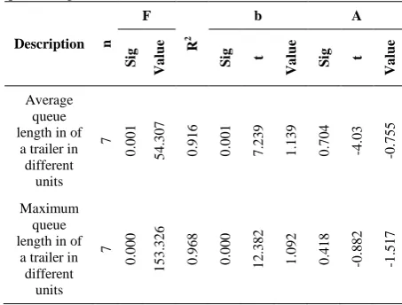
Finally, significance of the regression model examined that the results of average and maximum queue length is presented in Table 3.
According to the results presented in Table 2 indicate that the estimated model was a superior fit and a confidence level of 95% is significant. Thus, the model is attributable.
TABLE 2. Summary of t-test calculations for queue length of different units
Section T0
Critical Value
Test Result
Accumulation -1.46 1.71 Accept
North Entrance Storage 0.63 1.71 Accept
South Entrance Storage 1.57 1.71 Accept
Steel Material Storage 0.61 1.71 Accept
Warehouse of Bloom and Billet -1.29 1.71 Accept
Warehouse of Slabs -0.092 1.71 Accept
The door Number 2 1.48 1.71 Accept
TABLE 3. Regression analysis of average and maximum queue length
Description n
F
R
2
b A
S ig V a lu e S ig t V a lu e S ig t V a lu e Average queue length in of
a trailer in different units 7 0 .0 0 1 5 4 .3 0 7 0 .9 1 6 0 .0 0 1 7 .2 3 9 1 .1 3 9 0 .7 0 4 -4 .0 3 -0 .7 5 5 Maximum queue length in of
Since the number of samples in the regression model is not high enough, for closer examination comparisons between queue length of different units that recorded at certain intervals and simulation results was performed in 55 observed. The results of these observations are presented in Table 4.
As can be seen in Table 3, the regression model of queue length in different units reveals that the significance of the parameters is in accordance with the actual situation of the company.
3. 2. Validation of the Simulation Model in Case
Study In this study, validation is done with
expertise of the company. First, using animation and graphical representations, the movement of a trailer and queue length in different units are evaluated.
In order to test hypotheses, two criteria are used including: 1.Stay time of a trailer at company 2.Traffic volume of trailers on selected routes at the company. After data analysis, average stay time of trailer at the company was calculated based on: 1.Trailer that carrying raw materials and 2. Empty trailers that referring to loading productions.
Summary results of these calculations are as follows: The average presence time of trailer that carrying raw materials: 101 minutes
The average presence time of empty trailers that referring to loading productions: 172 minutes
Figures 4 and 5 show the diagram of presence time of trailer that carrying raw materials. In accordance with the histogram, maximum, mean and minimum stay time of trailer that carrying raw materials, respectively are 299, 107 and 14 minutes. 27% of trailers represents the highest frequency of batch trailer, related to trailers that between 54 to 74 minutes is present at the company. Also, it is observed that more than 50 percent of trailers are present more than 74 minutes at the company. This shows the long waiting times in queues of different units, which should reduce with increasing the number of services or decreasing the time of service.
The following results were obtained by performing the same analysis in the case of trailer that carrying products: maximum, mean and minimum spend time are respectively, 372,173 and 24 minutes.
TABLE 4. The results of observations- queue length of different units
n
F
R
2
b A
S
ig
V
al
u
e
S
ig t
V
al
u
e
S
ig t
V
al
u
e
55
0
.0
0
0
1
7
4
.1
6
4
0
.7
6
7
0
.0
0
0
1
3
.1
9
7
0
.8
9
6
0
.1
2
3
1
.5
6
6
1
.0
4
7
Figures 4. Histogram of presence time of trailer that carrying raw materials
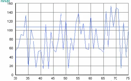
Figures 5. Presence time of trailer that carrying raw materials in the time of system stability
To determine the validity of the model, presence time of trailer at company is extracted from the output of the simulation model. The results of recorded data are shown in Figure 5.
Then, significant regression of models examined that is presented in Table 5. The results show that the model is significant at confidence level of 80%.
y=1.0029x-3.3975 R2=0.8064
TABLE 5. Regression analysis Diagram of presence time of trailers at company
n
F
R
2
b A
S ig V al u e S ig t V al u e S ig t V al u e 20 0 .0 0 0 7 .9 8 8 0 .8 0 6 0 .0 0 0 8 .5 5 0 1 .0 0 3 0 .5 2 1 -0 .6 5 5 -3 .3 9 7
The second criterion of validation model is comparing the trailer traffic volume with the statistics recorded in the simulation model. In order to increase the possibility of better analysis, corresponding points are plotted simultaneously on a graph for each path and regression line is calculated. The results of the regression model are presented in Table 6 which indicates the model is significant.
4. CONCLUSION AND FUTURE RESEARCHES
Most of the scheduling algorithms are designed to be established in an offline environment [17]. In this study, computer simulation models are discussed to optimize flexible manufacturing system (FMS) in one of the steel company. As the first step in modeling, knowledge of the system and the interactions between its components should be investigated, so source-destination traffic matrix of the company as the most important input of the simulation model to explaining the basic conceptual model has been developed.
After running the simulation model of sensitivity analysis to reduce the time of service units that have some problems such as long waiting time in the queue and queue length was conducted. Next, optimal number of service provider according to their facilities and service time per unit was calculated using the simulation model. According to a coefficient of model fitting, the results show that model has a high strength to rebuild the real system.
Finally, to determine flexible manufacturing system requirements for improving the existing and future situation, the following items are calculated:
TABLE 6. The results of the regression model of trailer traffic volume in the sample path
n
F
R
2
b A
S ig V al u e S ig t V al u e S ig t V al u e 30 0.00 0 295. 495 0.91 3 0.00 0 17.1 90 0.90 2 0.30 8 1.03 8 3.77 2
1. The optimal time service in each unit
2. Optimum number of service provider in each unit 3. Optimum number of domestic transportation fleet based on type
5. REFERENCES
1. Murr, L.E., "Computer simulation in materials science and engineering", Handbook of Materials Structures, Properties,
Processing and Performance, (2015), 1105-1121.
2. Liu, C.-H. and Huang, Y.-M., "An empirical investigation of computer simulation technology acceptance to explore the factors that affect user intention", Universal Access in the
Information Society, Vol. 14, No. 3, (2015), 449-457.
3. Tavakkoli-Moghaddam, R., Heydar, M. and Mousavi, S., "A hybrid genetic algorithm for a bi-objective scheduling problem in a flexible manufacturing cell", International Journal of
Engineering-Transactions A: Basics, Vol. 23, No. 3&4,
(2010), 235-252.
4. Principal, T. and Barnabas, K., "Optimization of minimum quantity liquid parameters in turning for the minimization of cutting zone temperature", International Journal of
Engineering-Transactions C: Aspects, Vol. 25, No. 4, (2012),
327-340.
5. Romashkin, A., Dub, V., Ivanov, I., Markov, S., Mal'ginov, A. and Tolstykh, D., "Development of an integral production process for manufacturing machinery billets based on computer simulation", Metallurgist, Vol. 58, (2015), 821-830.
6. Klos, S. and Trebuna, P., "Using computer simulation method to improve throughput of production systems by buffers and workers allocation", Management and Production Engineering
Review, Vol. 6, No. 4, (2015), 60-69.
7. Silva, C.E.S., Salgado, E.G., Mello, C.H.P., da Silva Oliveira, E. and Leal, F., "Integration of computer simulation in design for manufacturing and assembly", International Journal of
Production Research, Vol. 52, No. 10, (2014), 2851-2866.
8. Chramcov, B. and Bucki, R., "Lean manufacturing system design based on computer simulation: Case study for manufacturing of automotive engine control units", Design and
Management of Lean Production Systems, (2014).
9. Visuwan, D. and Phruksaphanrat, B., "Plant layout analysis by computer simulation for electronic manufacturing service plant",
World Academy of Science, Engineering and Technology, International Journal of Mechanical, Aerospace, Industrial,
Mechatronic and Manufacturing Engineering, Vol. 8, No. 3,
(2014), 586-591.
10. Azadeh, A., Keramati, A., Karimi, A., Sharahi, Z.J. and Pourhaji, P., "Design of integrated information system and supply chain for selection of new facility and suppliers by a unique hybrid meta-heuristic computer simulation algorithm",
The International Journal of Advanced Manufacturing
Technology, Vol. 71, No. 5-8, (2014), 775-793.
11. Oleskow-Szłapka, J. and Stachowiak, A., The use of computer simulation in warehouse automation, in Advances in sustainable and competitive manufacturing systems. (2013), 285-293.
12. Kermanpur, A., Varhraam, N. and Davami, P., "Computer simulation of equidxed eutectic solidifiction of metals",
International Journal of Engineering, Vol. 12, No. 4, (1999),
247-258.
14. Zahraee, S.M., Shariatmadari, S., Ahmadi, H.B., Hakimi, S. and Shahpanah, A., "Application of design of experiment and computer simulation to improve the color industry productivity: Case study", Jurnal Teknologi, Vol. 68, No. 4, (2014), 7-11. 15. Das, B., Garcia-Diaz, A., MacDonald, C.A. and Ghoshal, K.K.,
"A computer simulation approach to evaluating bowl versus inverted bowl assembly line arrangement with variable operation times", The International Journal of Advanced Manufacturing
Technology, Vol. 51, No. 1-4, (2010), 15-24.
16. Mukherjee, D. and Zohdi, T., "Computer modeling and simulation framework for particulate spray based manufacturing processes", in ASME 2013 International Mechanical Engineering Congress and Exposition, American Society of Mechanical Engineers., (2013), 15-21.
17. Namakshenas, M. and Sahraeian, R., "Real-time scheduling of a flexible manufacturing system using a two-phase machine learning algorithm", International Journal of
Engineering-Transactions C: Aspects, Vol. 26, No. 9, (2013), 1067-1076.
Optimizing Flexible Manufacturing System: A Developed Computer Simulation
Model
M. Nouri Koupaei, M. Mohammadi, B. Naderi
Department of Industrial Engineering, Faculty of Engineering, Kharazmi University, Tehran, Iran
P A P E R I N F O
Paper history: Received 21 March 2016
Received in revised form 23 April 2016 Accepted 02 June 2016
Keywords:
Flexible Manufacturing System Computer Simulation Modeling
Traffic Forecasting
ديكچ ه
عٌَت ذًاَتب ات تسا ُذض حزطه راساب یاّاضاقت ِب یخساپ ىاٌَع ِب زیذپ فاطعًا ذیلَت یاّ نتسیس زیخا یاّ لاس رد
ُزْب ،ذیلَت يیضاه سا بَلطه یرٍ یاّ نتسیس ِعسَت ٍ ذضر .ذّد صیاشفا ار تلاَصحه تذه ُاتَک یًاهس یاّ ُرٍد ٍ اّ
زتَیپهاک ار ىَگاًَگ تایلوع ماجًا یازب مسلا فاطعًا یاراد ٍ دایس رایسب یاّ تیلباق اب ییاّ يیضاه تخاس ىاکها ،ی
یبایسرا ٍ يیٍذت یازب یعطق یاّ نتیرَگلا ،لئاسه ًَِگٌیا یفداصت تیّاه ٍ یگذیچیپ لیلد ِب لاحٌیا اب .تسا ُدزک نّازف
یا رد .تسیً رادرَخزب مسلا ییاراک ٍ تقد سا اًْآ ذیلَت نتسیس یساس ٌِیْب یازب یزتَیپهاک یساس ِیبض شٍر سا ،ِلاقه ي
( زیذپ فاطعًا
FMS
،ذحاٍ زّ رد یّد سیٍزس ٌِیْب ىاهس :سا تسا ترابع ِلاقه يیا فاذّا .تسا ُذض ُدافتسا ) داذعت
ماگ رد .عًَ كیکفت ِب یلخاد لقًٍ لوح ىاگٍاً ٌِیْب داذعت ٍ ،ذحاٍ زّ رد اّ ُذٌّد تهذخ ٌِیْب اذبه سیزتاه ،تسخً
ىاهس یاّرایعه سا یداٌْطیپ لذه رابتعا یسرزب تْج يیٌچوّ .تسا ُذیدزگ ِئارا یهَْفه لذه حیزطت رَظٌوب ذصقه
يیا رد ار یساس ِیبض راشبا سا ُدافتسا ییاراک ٍ تقد یتابساحه جیاتً .تسا ُذیدزگ ُدافتسا ددزت نجح ٍ یّد سیٍزس
ذّد یه ىاطً لئاسه ًَِگ