SOLVING A STOCHASTIC CELLULAR
MANUFACTURING MODEL BY USING GENETIC
ALGORITHMS
M. J. Asgharpour and N. Javadian
Department of Industrial Engineering, Iran University of Science and Technology Tehran, Iran, [email protected]
(Received: December 4, 2002 – Accepted in Revised Form: February 26, 2004)
Abstract This paper presents a mathematical model for designing cellular manufacturing systems
(CMSs) solved by genetic algorithms. This model assumes a dynamic production, a stochastic demand, routing flexibility, and machine flexibility. CMS is an application of group technology (GT) for clustering parts and machines by means of their operational and / or apparent form similarity in different aspects of design and production. Most previous researches carried out in CMSs have been embodied in static production and deterministic demand states. Due to real situations of a CM model, it includes a great number of variables and restrictions requiring a long period of time, memory, and process power in order to be solved using available software packages and current optimal methods. Therefore, most researchers pay attention to novel methods. One of these methods is genetic algorithms (GAs). GA is a class of stochastic search techniques used for solving the NP-complete problems, such as CMSs. In this paper, a nonlinear integer model of CMS is designed in dynamic and stochastic states. Then, genetic algorithm is used to solve the problem and finally computational results are compared to existing optimal solutions in order to validate the efficiency of the proposed algorithm.
Key Words Cellular Manufacturing Systems, Mathematical Model, Dynamic and Stochastic States
(DSS), Dynamic and Deterministic States (DDS), Genetic Algorithms
ﻩﺪﻴﮑﭼ
ﻩﺪﻴﮑﭼ
ﻩﺪﻴﮑﭼ
ﻩﺪﻴﮑﭼ
ﺪﻣ ﻚﻳ ﻪﺋﺍﺭﺍﻪﺑ ﻪﻟﺎﻘﻣ ﻦﻳﺍ ﺪﻴﻟﻮﺗ ﻢﺘﺴﻴﺳﻲﺣﺍﺮﻃﻱﺍﺮﺑ ﻚﻴﺘﻧﮊﻢﺘﻳﺭﻮﮕﻟﺍ ﻪﻠﻴﺳﻭﻪﺑ ﻞﺣﻞﺑﺎﻗﻲﺿﺎﻳﺭ ﻝ
ﻲﻣﻲﻟﻮﻠﺳ ﺩﺯﺍﺩﺮﭘ
. ﻩﺪﺷﺎﻨﺑﻦﻴﺷﺎﻣﻭﻥﺎﻳﺮﺟﺮﻳﺬﭘﻑﺎﻄﻌﻧﺍﻭﻲﻟﺎﻤﺘﺣﺍﻱﺎﺿﺎﻘﺗ،ﺎﻳﻮﭘﺪﻴﻟﻮﺗﻱﺎﻨﺒﻣﺮﺑﺚﺤﺑﺩﺭﻮﻣﻝﺪﻣ
ﺖﺳﺍ . ﺹﺍﻮﺧﻪﺑﻪﺟﻮﺗﺎﺑﺎﻬﻨﻴﺷﺎﻣ ﻭﺕﺎﻌﻄﻗﻥﺁﺭﺩﻪﻛ ﺖﺳﺍﻲﻫﻭﺮﮔ ﻱﮊﻮﻟﻮﻨﻜﺗﺩﺮﺑﺭﺎﻛ ،ﻲﻟﻮﻠﺳﺪﻴﻟﻮﺗﻢﺘﺴﻴﺳ ﻭ
ﻲﻣ ﻱﺪﻨﺑ ﻢﻴﺴﻘﺗ ﻒﻠﺘﺨﻣ ﻱﺎﻫ ﻪﺘﺳﺩ ﻪﺑ ﺎﻬﻧﺁ ﻱﺮﻫﺎﻇ ﻞﻜﺷ ﺪﻧﻮﺷ
. ﻭﺖﺑﺎﺛ ﺪﻴﻟﻮﺗ ﺽﺮﻓ ﺎﺑ ﺮﻴﺧﺍ ﺕﺎﻘﻴﻘﺤﺗ ﺮﺘﺸﻴﺑ
ﺖﺳﺍ ﻪﺘﻓﺮﻳﺬﭘﻡﺎﺠﻧﺍﻦﻴﻌﻣﻱﺎﺿﺎﻘﺗ .
ﻥﺎﻣﺯﻪﻛﺖﺳﺍﻱﺭﺎﻴﺴﺑﻱﺎﻬﺘﻳﺩﻭﺪﺤﻣﻭﺎﻫﺮﻴﻐﺘﻣﻞﻣﺎﺷﻪﻟﺎﺴﻣﻲﻠﻤﻋﺖﻟﺎﺣﺭﺩ
ﺩﻮﺧ ﻪﺑﻲﻠﻌﻓ ﻱﺯﺎﺳﻪﻨﻴﻬﺑ ﻱﺎﻫﺭﺍﺰﻓﺍ ﻡﺮﻧﺯﺍ ﻩﺩﺎﻔﺘﺳﺍﺎﺑﺍﺭ ﻱﺩﺎﻳﺯﻪﻈﻓﺎﺣ ﻭ
ﻲﻣﺹﺎﺼﺘﺧﺍ ﺪﻫﺩ
. ﺕﺎﻘﻴﻘﺤﺗﻦﻳﺍﺮﺑﺎﻨﺑ
ﻚﻴﺘﻧﮊﺵﻭﺭﺪﻨﻧﺎﻣﻥﺁﻞﺣﻦﻳﻮﻧﻱﺎﻬﻤﺘﻳﺭﻮﮕﻟﺍﻪﺋﺍﺭﺍﻪﺑﺍﺭﺩﻮﺧﺰﻛﺮﻤﺗﺪﻳﺪﺟ )
GA (
ﺪﻧﺍﻩﺩﺍﺩﺭﺍﺮﻗ .
ﺵﻭﺭ
GA
ﻚﻳ
ﻞﺋﺎﺴﻣ ﻞﺣﻱﺍﺮﺑ ﻪﻛﺖﺳﺍ ﻲﻟﺎﻤﺘﺣﺍﻱﻮﺠﺘﺴﺟ ﻚﻴﻨﻜﺗ
NP-complete
ﻲﻣ ﻩﺩﺎﻔﺘﺳﺍ ﺩﻮﺷ
. ﻝﺪﻣ ﻚﻳﻪﻟﺎﻘﻣ ﻦﻳﺍ ﺭﺩ
ﻞﺣﻱﺍﺮﺑﺢﻴﺤﺻﺩﺪﻋﻲﻄﺧﺮﻴﻏﻱﺰﻳﺭﻪﻣﺎﻧﺮﺑ ﻪﻟﺎﺴﻣ
CMS
ﺖﺳﺍﻩﺪﺷﻞﺣﻚﻴﺘﻧﮊﻢﺘﻳﺭﻮﮕﻟﺍﺯﺍﻩﺩﺎﻔﺘﺳﺍﺎﺑﻭﻪﺋﺍﺭﺍ .
ﺖﺳﺍﻩﺪﻳﺩﺮﮔﻪﺴﻳﺎﻘﻣﻪﻨﻴﻬﺑﺏﺍﻮﺟﺎﺑﻝﺪﻣﻲﻳﺍﺭﺎﻛﻦﻴﻴﻌﺗﺭﻮﻈﻨﻣﻪﺑﻞﺻﺎﺣﺏﺍﻮﺟﺖﻳﺎﻬﻧﺭﺩ .
1. INTRODUCTION
In most CMSs, the production is dynamic in practice because the variability in demand. In other words, the production programming cycle can be divided into several periods (i.e. multi-period) when the demand for part types is changing from one period to another. In this case, by assuming the
for forecasting the stochastic part demand. CMS model in this paper is considered for the dynamic case and the demand is stochastic with specific probability distribution for each part type in each period. It is called dynamic and stochastic states (DSS).
Short production life cycles, high production variety, unpredictable demand, and short delivery times have caused manufacturing systems to operate under dynamic and uncertain environment these days. Several efforts in different research areas such as dynamic plant layouts [3, 4], flexible plant layouts [2, 5], and dynamic cellular manufacturing [1, 4] have been proposed to deal with these dynamic and stochastic production requirements. Chen [1] developed a mathematical programming model for a system reconfiguration in a dynamic cellular manufacturing environment. Song and Hitomi [6] developed a methodology to design flexible manufacturing cells. Wicks [4] proposed a multi–period formation of the part family and machine cell (PF/MC) formation problem. Seifoddini [7] presented a probabilistic machine cell formation model to deal with the uncertainty of the product mix for a single period. Harhalakis et al, [8] presented an approach to obtain robust CMS designs with satisfactory performance over a certain rang of a demand variation. Mungwatanna [27] presented a CMS model by assuming routing flexibility in dynamic and stochastic production requirements.
Base of genetic algorithms (GAs) in natural evolution studies the transformation of the organism type for more adaptation to its environment. In spite of other stochastic search methods, GAs searches the feasible space by the set of feasibility solutions simultaneously in order to find optimal or near-optimal solutions. The procedure is carried out by the use of genetic operations. This paper develops and uses GAs for a CMS model in the DSS cases with the objective function to minimize the production costs. Finally the computation results are promising. The format of the paper is as follows: Section one, as above, introduced some of the models of CMS solved by GAs and reviews the literature on the CMS problem. The CMS model in DSS is described in Section 2. The procedure for developing GAs is discussed in six subsections of Section 3. The implementation of GAs for the CMS model is demonstrated in Section 4. Section
5 contains the final conclusions.
2. CMS MODEL IN DSS
The dynamic and stochastic states (DSS) are the expansion of the dynamic and deterministic states (DDS) in which the demand of each part type in each period is considered as a random variable with specific probability distribution. In this way, the demand optimal value for each part type in each period must be determined in a specific confidence level minimizing the objective function. Thus, a confidence interval of 95% is considered for the demand of each part type in each period. Then the absolute sum of demand means deviation for all part types in all periods are added to objective function as a penalty. Finally, confidence interval’s lower and upper bounds is added to the model as a restriction. The CM model assumes the existence of operation sequence, routing flexibility, machine flexibility, and the ability of inter-cell relocation of machines. This model must satisfy the following expectations:
1. Establishing parts family and machine groups
simultaneously.
2. Choosing a process plan for each part type with
at least inter-cell and intra-cell material handling costs in each period by assuming the existence of several alterative process plans for each part type.
3. Estimating the optimal demand for part types in
such a way that it has the least difference to its expected value.
4. Purchasing inter-cell relocation of machines as
a necessity when the demand for parts is changed between periods.
2.1. Assumptions
The assumptions of the model are as follows:1. The operating times for all part type operations on different machine types are known.
2. The demand density function for each part type in each period is known.
3. The capabilities and capacity of each machine type are known and constant over time.
4. Investment or purchase cost per period to procure one machine of each type is known.
5. Operating cost of each machine type per hour is
6. Parts are moved between and inside of cells in
batches. The inter-call and intra-cell material handling cost per batch between and inside of cells is known and constant (independent of quantity of cells)
7. The number of cells used must be specified in advance and it remains constant over time.
8. Bounds and quantity of machines in each cell need to be specified in advance and they remain constant over time.
9. Machine relocation from one cell to another is performed between periods and it requires zero time.
10. The machine relocation cost of each machine
type is known and it is independent of where machines are actually being relocation.
11. Each machine type can perform one or more
operations (machine flexibility). Likewise each operation can be done on one machine type with different times (routing flexibility).
12. Inter-cell and intra-cell handling costs are
constant for all moves regardless of the distance traveled.
13. No inventory is considered. 14. Setup times are not considered.
15. Backorders are not allowed. All demand must
be satisfied in the given period.
16. No queuing in production is allowed. 17. Machine breakdowns are not considered. 18. Processing capabilities are 100% reliable (i.e.
no rework / scrap).
19. Batch size is constant for all productions and all
periods.
20. Machines are available at the state of the period
(zero installation time).
21. The time value of money is not considered in
the CMS model.
2.2. Design Objectives
Multiple costs must be considered in the design objective in an integrated manner. All costs involved in the design of CMSs must be incorporated. However, it is not possible to consider all costs in the model due to the complexity and computational time required. In this paper, costs are limited to those, which are also related to dynamic and stochastic production environments and the use of routing and machine flexibility. The objective is to minimize the sum of the following costs:1. Machine cost: The investment or purchase cost
per period to procure machines. This cost is calculated based on the number of machines of each type used in the CMS for a specific period.
2. Operating cost: The cost of operating machines for producing parts. This cost depends on the cost of operating each machine type per hour and the number of hours required for each machine type.
3. Inter-cell and intra-cell material handling costs: The cost of transferring parts between and inside of cells when parts cannot be produced completely by a machine type or in a single cell. This cost is incurred when batches of parts have to be transferred between machines in a cell or between cells. Inter-cell moves, decreases the efficiency in the CMS by complicating production control and increasing material handling requirements and flow time.
4. Machine relocation cost: The cost of relocating
machines from one cell to another between periods. In dynamic and stochastic production environments, the best CM design for one period may not be an efficient design for subsequent periods. By rearranging the manufacturing cells, the CMS can continue operating efficiently as the product mix and demand change. However, there are some drawbacks with the rearrangement of manufacturing cells. Moving machines from cell to cell requires effort and can lead to the disruption of production.
5. Deviation of mean penalty for part types
demand: The absolute sum of deviation of mean for part types demand in all periods. In stochastic demand state, if possible, the difference between the estimation value of demand for each part type and its expected value must be the least.
2.3. System and Input Parameters
The input parameter values must be supplied for each period in the planning horizon.1. Part types (product mix): A set of part type to be produced in the CMS in each period. The product mix varies from period to period as new parts are introduced and old parts are discontinued.
2. Part types demand probability distribution: The
specific probability distribution for each part type in each period, through introduction of mean and standard deviation of distribution by assuming that the parts demand probability distribution is one of three binomial, normal or β distributions.
3. Operating sequence: An ordered list of operations
4. Operating time: Time required by a machine to
perform an operation on a part type.
5. Machine type capability: The ability of a
machine type to perform operations.
6. Machine type capacity: The amount of the time a machine of each type is available for production in each period.
7. Available machines: The available machines are the set of machines that will be used to form manufacturing cells. The necessary number of each machine type is specified by the model.
2.4. Constraints
The following constrains must be imposed in the model:1. There must be sufficient machine capacity to
produce the specified product mix in each period.
2. Cell size must be specified. Upper and lower
bounds can be used instead of a specific number.
3. The number of cells in the system must be
specified.
4. The confidence level for the part types probability
demand must be specified. Managers or designers can specify this information.
2.5. Notation
The notation of the model is presented as follows:2.5.1. Indices
c index for manufacturing cells (c=1,…,C) m index for machine types (m=1,…,M) p index for part types (p=1,…,P) h index for time periods (h=1,…,H)
j index for operations required by part p (j=1,…,Op)
2.5.2. Input Parameters
tjpm time required to perform operation j of part
type p on machine type m.
EDph mean of the probability distribution for part
type p in period h.
SDph standard deviation of the probability distribution
for part type p in period h.
The EDph and SDph parameters are entered by
means of three distributions as following:
I - The normal distribution: by assuming in this case that the demand is continuous, and EDph equal
the mean of distribution (EDph=µ) and SDph equal
the standard deviation of distribution (SDph=δ)
II - The binomial distribution: by assuming in this case that the demand is ruptured, the EDph and SDph parameters are countered by means of the
probability of demand for each part p(θ) and the number of production for part p(n) as the following:
EDph = nθ (1)
)
1
(
n
SD
ph=
θ
−
θ
(2)III – The Beta distribution: in this case, The EDph and SDph parameters are countered by means of the
most optimistic value of the demand (H), the most possible value of the demand (M) and the most pessimistic value of the demand (L) for part p as the following:
6
H
M
4
L
ED
ph=
+
+
(3)6
L
H
SD
ph=
−
(4)B batch size for inter-cell and intra-cell material handling
αm purchase cost of type m machine
βm Operating cost per hour of type m machine
γ intercell and intra-cell material handling cost per batch
δm relocation cost of type m machine
Tm capacity of each of type m machine (hours)
LB lower bound cell size UB upper bound cell size
=
otherwise
0
m
type
machine
on
done
be
can
p
part
of
j
operation
if
1
a
jpm2.5.3. Decision Variables
Nmch number of machines of type m used in cell c
during period h
otherwise
0
h
period
in
c
cell
in
m
type
machine
on
done
is
p
type
part
of
j
operation
if
1
X
jpmchK+
mch number of machines of type m added in cell
K
-mch number of machines of type m removed
from cell c during period h
XDph number of demand for part type p in period
h
Vmh number of type m machine existing in store
(remainder cell) in period h
When the number of periods is more than two periods, it is possible that some of the machines are not used in middle periods (for example, machine
m is used in periods 1,3 and not used in period 2). Thus, for avoidance of crowding of the machines in cells (and excess of machines from over upper bound cell size (UB)), it is necessary that the idle machines be removed to a figurative store or remainder cell (the relocation cost of machines form/to store not to take into account). Thus, the introduced variable Vmh is used as a memory. It
means, when a machine type in a period is needed, the first one is searched in memory and if not founded, it must be purchased. The Vmhvariable is countered as following:
+
−
=
∑
∑
= + = − − C 1 c mch C 1 c mch ) 1 h ( mmh
max
0
,
V
K
K
V
(5) As a result, the following constraints must be
added to the model:
0
V
mh≥
(6)h
m,
K
K
V
V
C 1 c mch C 1 c mch ) 1 h ( mmh
≥
+
∑
−
∑
∀
= +
= −
− (7)
2.6. Mathematical Formulation
The mathematical formulation for the design of CMSs is developed such that part families and machines groups are formed simultaneously. The simultaneous machine– part grouping strategy generally yields better results than those of sequential strategies (part grouping and then machine grouping or reversal process), since all the decisions are made at the same time. However, it can be more complicated to be modeled and results in a large mathematical formation, which requires a substantial amount of time to be solved. Using the above notation, the objective function and constraints are as follows:∑∑∑∑∑
∑
∑∑
∑
= = = = = − = − = = = β + + − + α = H 1 h C 1 c M 1 m P 1 p Op 1 j m jpmch jpm ph ) 1 h ( mc C 1 c ) 1 h ( mc H 1 h M 1 m mh C 1 c mch m x t XD V N V N Z min (8) h p, j, 1 x a C 1 c M 1m jpm jpmch
∀ =
∑∑
= = (I)h
mc,
N
T
x
t
XD
m mchP
1 p
Op
1
j ph jpm jpmch
∀
≤
∑∑
= = (II)h c, LB K K N M 1 m mch M 1 m mch M 1 m mch ∀ ≥ − +
∑
∑
∑
= − = + = (III) h c, UB K K N M 1 m mch M 1 m mch M 1 mmch +
∑
−∑
≤ ∀∑
= − = + = (IV) h c, m, N K KNmc(h 1) + mch+ − mch− = mch ∀
− (V)
h
m,
K
K
V
V
C 1 c mch C 1 c mch ) 1 h ( mmh
≥
+
∑
−
∑
∀
= +
= −
− (VI)
(
V
V
)
m,
h
K
R
C mh m(h 1)1 c
mch
mh
≤
+
−
−∀
=+
∑
(VII)(
V
V
)
m,
h
K
R
C m(h 1) mh1 c
mch
mh
≤
+
−−
∀
=−
∑
(VIII)h
p,
SD
96
.
1
ED
XD
ph≥
ph−
ph∀
(IX)h
p,
SD
96
.
1
ED
XD
ph≤
ph+
ph∀
(X)Integer and 0 XD , R , V , K , K , N , 1 or 0 x ph mh mh mch mch mch jpmch ≥ = − +
inter-cell and intra-cell material handling costs, the machine relocation cost and the absolute sum of the demand deviation from mean for part types over the planning horizon. The first term represents the cost of all machines required in the CMS. The machine purchase or investment cost is obtained by the difference between sum of the number of machines of each type in all cells and their number in store in current and pervious periods in relation to their respective costs. The second term is the cost of operating machines; It is the sum of the operating cost of the number of hours of each machine type. The third term is the inter-cell and intra-cell material handling costs. The total of this cost is obtained using the number of inter-cell and intra-cell transfer for each part type and the cost of transferring a batch of each part type. The next cost is the machine relocation cost. It is the sum of the cost of the number of machined relocated (Rmh).
The number of machined relocated (Rmh) is
obtained by term 10 .The last term is the penalty of demand deviation from mean for all part types. This cost is obtained by the absolute sum of the deviation of demand mean for all part types over the planning horizon.
Constrain I ensures that each part operation is assigned to one machine and one cell. Constrain II ensures that machine capacities are not exceeded and can satisfy the demand. Constrains III and IV specify the lower and upper bounds of cells. Constrain V ensures that the number of machines in the current period is equal to the number of machines in the previous, plus the number of machines being moved in and minus the number of machines being moved out. In order words, they ensure conservation of machines over the horizon. Constrain VI by term of 6 ensures that the number of machines in the store in the current period is equal to the number of machines in the store in the previous, plus the number of machines being moved out of cells and minus the number of machines being added to cells. Constrains VII and VIII by term of 10 ensure that the number of machines relocation is equal to minimum value between the number of machines being added to cells and the number of machines being moved out of cells, irrespective of the relocations from or to the store. Constrains IX and X ensure that the optimal demand for part types are not exceeded from the confidence interval’s lower and upper
bounds in level 95%.
3. A GENETIC ALGORITHM FOR SOLVING THE CMS MODEL IN DSS
Holland and his associates at the university of Michigan developed genetic algorithms (GAs) initially in the 1960s and 1970s. The first full and systematic (and mainly theoretical) treatment was contained in Holland’s book [9]. Goldberg gave an interesting survey of some practical work carried out in this era [10]. Among these early applications of GAs were those developed by Bagley for a game–playing program [11], by Rosenberg in simulating biological process [12], by Cavicchio for solving pattern–recognition problems [13], by Goldberg and Lingle; Grefenstette; Van Gucht; and Whitley et al. for TSP problems [14], [15], [16], [17], by Rinooy Kan; Reeves; Ackley for Sequencing and Scheduling problem [18], [19], [20], [21], by Dawis for Graph coloring problems [22] by Goldberg and Smith for solving a Knapsack problem [23], [24] and by Joines and Culbreth and King for CMS [25], [26].
In this section, a genetic algorithm is introduced for solving the described CMS model in Section 2. In designing GAs, six principle factors must be considered as explained below:
3.1. Solution Coding (Chromosome Structure)
A chromosome or feasible solution proportional to the described CMS model must consist of the following genes in each period:1. The gene related to the assignment of part operation to machine is named Matrix [Xij] where;
i = 1, 2, …, P, j = 1, 2, …, r; P = the number of part types and r is defined in term of 11; Opi = the
number of operations of part i). The alleles are limited to 0, 1, 2, …, M (M = the number of machines). For example, the term of X12 = 4 means
that the operation 2 of part 1 is assigned to machine 4 (if a214 = 1).
{ }
i p1 i
Op
MAX
r
=
= (11)2. The gene related to the assignment of the part operation to cell is named Matrix [Yij]. The alleles
cells). For example, the term of Y12 = 3 is means
that the operation 2 of part 1 is assigned to cell 3. 3. The gene related to the number of machines being available in each cell is named Matrix [Nmc]
where; c = 1, 2, …, C and m = 1, 2, …, M. The alleles are limited to 0, 1, … . For example, the term of N52 = 1 is means that the number of
machine 5 in cell 2 is equal to 1. By considering constrains III and IV in the model, the term of 12 must be established.
h
c,
UB
N
LB
M 1 m mch∀
≤
≤
∑
= (12)4. The gene related to the number of machines
being moved in each cell or the number of machines being moved out is named Matrix [Kmc].
The alleles are limited to … , -2, -1, 0, 1, 2, … . For example, the term of K52 = 1 means that the
number of machine 5 that is moved to cell 2 is equal to 1 and the term of K52 = -1 means that the
number of machine 5 that is moved out cell of 2 is equal to 1.
5. The gene related to the estimated demand for
part type is named Vector [Di]. The alleles are
limited to the lower and upper bounds of confidence interval for the part demand. For example, the term of D6 = 580 means that the amount of demand for
part 6 is equal to 580.
In general by combining four matrices and one vector described above, the chromosome structure in each period is obtained as Figures 1 or 2. It is clear that each chromosome or feasible solution consists of the H structure as shown in Figure 1 or 2, where H is the number of periods.
3.2. Generation of initial population
A sequential strategy is used for obtaining the initial population. In this strategy, the numbers of LB machines are first assigned to each cell randomly. Then the operations related to each part type are assigned to machines existing in cells randomly by means of ajpm values. Asrequired, the new machines are assigned to cells or relocated between them. If possible, each operation must be assigned to the cell that the pervious operation being assigned. For transforming an infeasible solution to feasible one, a new procedure called “Filter” is introduced. The solutions, which cannot transform to feasible ones, must be eliminated. For avoiding the monotony or lack of the variety in generations, each new solution is compared with another solutions produced recently in respect to its similarity. If the similarity between the new solution and another solution is less than the specific value, it is accepted, otherwise it will be eliminated. The similarity between two solutions (chromosomes) is defined as follows: ) M , P ( Max ) C r ( 2 B a
Sij ij
× + ×
−
= (13)
where aij is the number of genes consisting of the
same allele in chromosome i and chromosome j. The B variable is called the diagonal value. This variable is equal to the number of genes that always consists of zero allele in both chromosomes, due to the lack of the demand for some part types or shortage of the number of operations of some part type as compared with r value (see term of 11) or the barren genes are obtained from different between P and M. The B variable is obtained form term of 14. The term of
)
M
,
P
(
Max
)
C
r
(
2
×
+
×
demonstrates the area of the chromosome structure.(
)
(
)
− + − + − =∑
= ) M , P min( ) M , P max( a r ) e 1 ( OP r e 2 B P 1 i i ii (14)
where; otherwise 0 nonzero be i part for demand the if 1 ei
[ ] [ ] [ ] [ ]
[
X
p×r|
Y
P×r|
K
M×C|
N
M×C|
[
D
]
p×1]
Figure 1. Chromosome macros copy structure.
p 2 1 MC M2 M1 2C 22 21 1C 12 11 MC M2 M1 2C 22 21 1C 12 11 pr p2 p1 2r 22 21 1r 12 11 pr p2 p1 2r 22 21 1r 12 11 D D D N .. N N N ... N N N ... N N k .. k k k ... k k k ... k k y ... y y y ... y y y ... y y x ... x x x ... x x x ... x x M M M M M
< = >
M P if r
M P if 0
M P if C a
3.3. Fitness Evaluation with Objective Function
The fitness is a criterion for the quality measurement of a chromosome or feasible solution. By considering the explained CMS model, an offspring or new solution is accepted when its objective function value is minimum as compared with their parents. Thus, the fitness function is the same objective function presented in the CMS model.3.4. Mating Pool Selection Strategy
For creating the new generation, it is necessity that some of the chromosomes with the latest fitness in the current generation are selected for recombining or creating chromosomes related to the new generation. In this case, a normalized fitness strategy is used in which the fitness of current generation chromosomes are first normalized according to term of 15. Then the chromosomes, that their normalized fitness are less or equal to zero, are selected as a mating pool.K 1,2,..., i
; f
Z i
i =
δ µ −
= (15)
where, Zi is the normalized fitness of chromosome
i and fi is the fitness of chromosome i. µ is the
mean of chromosomes fitness and δ is a standard deviation of chromosomes fitness in the current generation.
3.5. Improved GA Operators
In this paper, the chromosome structure is formed as a matrix. Thus, the GA linear operators cannot be used to a matrix type as a traditional form. These operators must be improved proportional to the matrix type. Therefore by attention to the nature of the matrix, for each of three operators called crossover, mutation, and inversion is considered as four cases named columnar, linear, diametric, and districted. In each repeat, one of operations is exercised over one of the matrices [X] or [Y] and/or [N] related to the current chromosome as one of four cases above randomly then the matrix [K] that is up to date by means of matrix [N]. The cases of columnar, linear, diametric, and districted are described asfollows:
1. Exercising of operation as columnar In this case, two numbers are first selected randomly in the relevant matrix row limits. Then the operation is exercised over obtained columns.
2. Exercising of operation as linear In this case, two numbers are first selected randomly in the relevant matrix columnar limits. Then the operation is exercised over obtained rows.
3. Exercising of operation as diametric In this case, two numbers in the relevant matrix columnar or row limits and one of the directions of primary or secondary are selected randomly. Then the operation is exercised over obtained diameters. 4. Exercising of operation as described In this case, two numbers in the relevant matrix columnar limits and also two numbers in relevant matrix row limits are selected randomly. Then the operation is exercised over obtained district.
3.5.1. Arithmetic Crossover Operators
Arithmetic crossover operators [25] and [26] products two complimentary linear combinations of the parents, where r = U (0,1).a -1 b , 1 a 0 ; aP bP C
bP aP C
2 1 2
2 1 1
= ≤ ≤
+ =
+
= (16)
where, C1 and C2 are offspring of P1 and P2. To
achieve the necessary integer representation of the variables, the following equation is performed.
≤ +
> +
= +
ij ij ij
ij
ij ij ij
ij ij
ij a[P] b[P] if[P] [P]
P] [ [P] if ] P [ b ] P [ a ] P [ b ] P [ a
(17)
3.6. Stopping Criterion
For stoppingthe algorithm, the following criterions are considered.
1- Number of generations In this case, the algorithm terminates if the number of generations is exceeding of the specific number.
4. COMPUTATIONAL RESULTS
The presented model in DSS is solved by the following assumptions:
3
C
and
2
H
;
3
P
O
;
10
M
;
12
P
≥
≥
≤
=
=
including 2412 linear variables, 1352 nonlinear variables, 234 linear constrain and 63 nonlinear
TABLE 1. Comparison of GA Solution to Optimal Solution in DDS.
Costs
Approach
Objective function
Equipment or Purchasing
cost
Operating cost
Material handling
cost
Relocation
cost Time
Different
(percentage) Dimension of test problem
Lingo6 34972 8686 14828 11458 0 00:02:18 0 % GA 35203 8686 15605 10913 0 00:07:18 0.6 %
8×6 H=2,C=3 Lingo6 45772 7745 25970 12056 0 00:07:10 0 %
GA 45772 7745 25970 12056 0 00:16:01 0 %
10×8 H=2,C=3 Lingo6 35071 8022 14734 12314 0 00:03:15 0 %
GA 35279 8022 14240 13018 0 00:25:09 0.6 % 11×8 H=2,C=3 Lingo6 35945 8706 15787 11452 0 01:15:59 0 %
GA(K=100) 36645 8706 16059 11880 0 00:23:14 1.9 % GA(K=200) 36373 8706 15787 11880 0 00:13:05 1.1 %
11×9 H=2,C=3 Lingo6 83889 13239 48663 21986 0 04:58:51 0 %
GA 84662 13239 48663 22720 0 00:00:00 0.8 % 12×10 H=3,C=3
TABLE 2. Comparison of GA Solution to Optimal Solution in DSS.
Costs
Approach
Objective Function
Purchase cost
Operating Cost
Material handling cost
Relocation cost
Sum of M.D
demand Time
Standard deviation
Different (percentage)
Dimension of test problem
Lingo6 23530 5240 11031 7156 0 102 00:10:17 - 0% GA 25087 6280 11031 7560 0 1 00:00:59 - 6.6%
5×4 H=2,C=2
Lingo-LB 43123 5564 19452 18123 0 - - 5716 0% GA 43706 53780 18405 19200 0 432 00:04:21 - 16%
6×5 C=2,H=2
Lingo-LB 50512 12200 29226 9086 0 - - 1698 0% GA 49473 12200 27815 9320 0 138 00:01:14 - 1%
8×6 H=2,C=3
Lingo-LB 44452 9986 19073 15393 0 - - 3443 0% GA 28027 9420 19647 18640 0 319 00:25:31 - 17%
9×7 H=3,C=3
Lingo-LB 33971 8650 2702 12619 0 - - 581 0% GA 34241 8650 12572 12960 0 60 00:18:14 - 2%
11×8 H=3,C=3
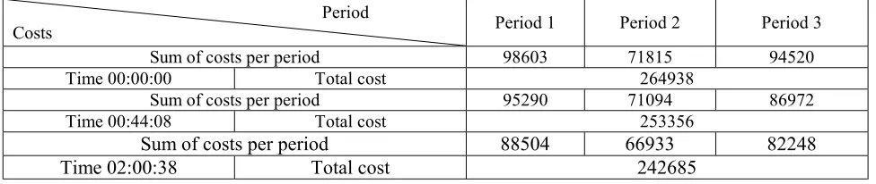
TABLE 3. The GA Solution for a Typical Problem (20×15) with H=3, C=3 in DSS.
Period
Costs Period 1 Period 2 Period 3
Sum of costs per period 98603 71815 94520
Time 00:00:00 Total cost 264938
Sum of costs per period 95290 71094 86972
Time 00:44:08 Total cost 253356
Sum of costs per period 88504 66933 82248
constrains through a PC–Pentium III 1.1 Gz and Lingo 6 software. As a result, for comparing the GA solution with the optimal solution, five test problems in dynamic-deterministic states and five test problems in dynamic-stochastic states are solved in dimensions less than the assumptions above by the GA program and Lingo, Then the obtained results have been compared as shown in Tables 1 and 2. Assuming Beta distribution conditions, lower bound (LB) solution is used; because the model in DSS is extremely nonlinear. By considering the validity of the GA program in high dimensions, a typical test problem is solved by GA assuming
;
15
M
;
20
P
=
=
O
P
=
3
;
H
=
3
;
and
C
=
3
where the demand of part types is according to Beta distribution, as illustrated in Table 3. In high dimensions, the rate of convergence for the algorithm and the computational time to best solution is carried out. All above test problems have been generated randomly by a computer within the specific limits.By having considered the proposed CM model, the GA program is able to find and report the near-optimal and promising solutions in a good reasonable time. This indicates the success of the proposed algorithm. In general, the obtained results can be
divided into the following parts:
1. In DDS with low dimension, the different mean between the GA solution and the optimal solution is +0.62% where the GA program finds the near-optimal solution in a less computational time than the optimal algorithm.
2. In DSS and low dimensions, the different mean between the GA solution and the optimal solution is +8.52% where the GA program finds the near-optimal solution in a less computational time than the optimal algorithm. Because of using the lower bound (LB) solution, the time measurement for the optimal solution is impossible. The reason is that the model in DSS is extremely nonlinear and the achievement time of finding the optimal solution is certainly more than the GA solution.
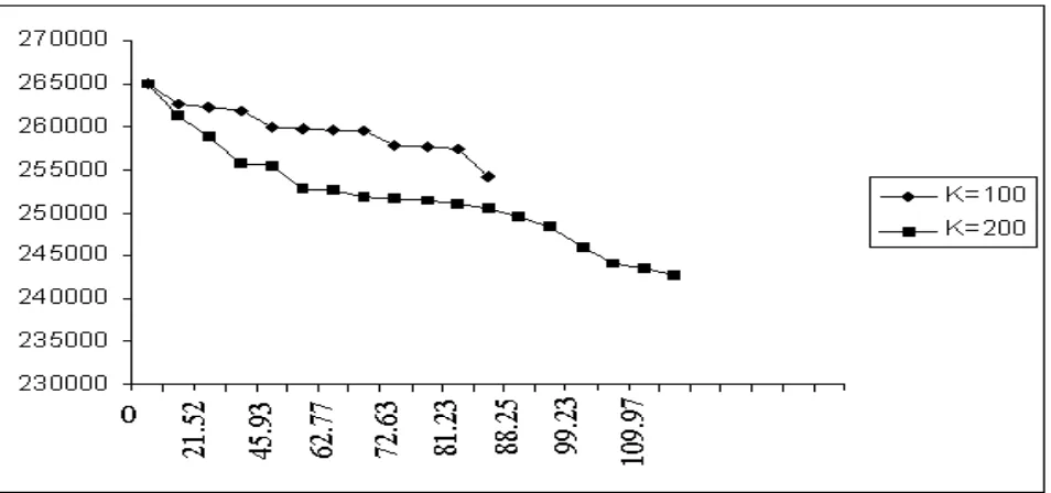
3. In DDS and DSS with high dimensions, solving the model by PC is practically impossible in terms of time consuming. However, the GA program reports some acceptable solutions in logical time. The convergence rate of the GA program (based on objective cost and process time) for problem 20×15 in DSS is shown in Figure 3 by means of two different population sizes. When the size of population (K) increases from 100 to 200, the
convergence rate and the objective function value are improved. Of course, this manner is not always truthful.
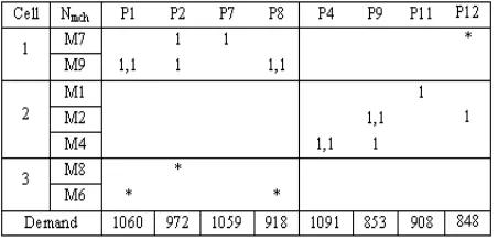
4. According to the GA program, the optimal number of cells is specified automatically. Whereas, in the proposed model, the number of cells must be specified and fixed from the outset. For example in Figure 4, no part type is assigned to cell 3. Thus, the number of cells will be reduced to two cells by moving machines M8 and M6 to cell 1.
5. Because of using the simultaneous machine– part grouping strategy and the definition of Xjpmch variable, one of drawback points of the
proposed model is to consider intra-cell material handling cost. For avoiding this drawback, the Xjpmch variable must be broken into two Xjpch
and Yjpmh variables. However, this procedure
forces the model being a nonlinear one extremely. Whereas, the above procedure is not difficult for the GA approach. In other words, the proposed GA approach can ignore intra-cell material handling cost.
5. CONCLUSION
The GA program finds and reports the near optimal and lower bound solutions in shorter time interval, on the average, rather than their optimal solutions in all test problems using both DDS and DSS. The solutions obtained by the GA program are getting more credit and justification for real-world condition. In general, improving the GA principle presented by six factors will increase the probability of achievement to optimal solution.
6. REFERENCES
1. Chen, M., “A Mathematical Programming Model for Systems Reconfiguration in a Dynamic Cellular Manufacturing Environment”, Annals of Operations Research, 77 (1), (1998), 109-128.
2. Benjaafar, S. and Sheikhzadeh, M., “Design of Flexible Plant Layouts”, IIE Transactions, to be Appeared. 3. Montreuil, B. and Laforge, A., “Dynamic Layout Design
Given a Scenario Tree of Probable Futures”, European Journal of Operational Research, 63, (1992), 271-286. 4. Wilhelm, W., Chiou, C. and Chang, D., “Integrating
Design and Planning Considerations in Cellular Manufacturing”, Annals of Operations Research, 77 (1), (1998), 97-107.
5. Yang, T. and Peters, B., “Flexible Machine Layout Design for Dynamic and Uncertain Production Environments”,
European Journal of Operational Research, 108, (1998), 49-64.
6. Song, S. and Hitomi, K., “Integrating the Production Planning and Cellular, Layout for Flexible Cellular Manufacturing”, Production Planning and Control, 7 (6), (1996), 585-593.
7. Song, S. and Hitomi, K., “Integrating the Production Planning and Cellular, Layout for Flexible Cellular Manufacturing”, Production Planning and Control, 7 (6), (1996), 585-593.
8. Harahalaks, G., Nagi, R. and Proth, J., “An Efficient Heuristic in Manufacturing Cell Formation to Group Technology Applications”, International Journal of Production Research, 28 (1), (1990), 185-198.
9. Holland, J. H., “Adaptation in Natural and Artificial Systems”, University of Michigan Press, Ann Arbor, (1975).
10. Goldberg, D. E., “Genetic Algorithm in Search Optimization and Machine Learning”, Addison-Wesley, Reading, Mass., (1989).
11. Bagley, J. D., “The Behavior of Adaptive Systems Which Employ Genetic and Correlation Algorithms”, Doctoral Dissertation, University of Michigan, (1976).
12. Rosenberg, R. S., “Simulation of Genetic Population with Biochemical Properties”, Doctoral dissertation, University of Michigan, (1967).
13. Cavicchio, D. J., “Adaptive Search Using Simulated Evolution”, Doctoral dissertation, University of Michigan, (1972).
14. Goldberg, D. E. and Lingle, R., “Alleles, Loci and the Traveling Salesman Problem”, (1985), 154-159.
15. Suh, J. Y. and Van Gucht, D., “Incorporation Heuristic Information into Genetic Search”, (1987), 100-107. 16. Grefenstette, J. J., “Incorporating Problem – Specific
Knowledge into Genetic Algorithms”, (1987), 42-60. 17. Whitley, D., Starkweather, T. and Shaner, D., “The
Traveling Salesman Problem and Sequence Scheduling Quality Solutions Using Genetic Edge Recombination”, (1991), 350-372.
18. Reeves, C. R., “A Genetic Algorithm for Flowshop Sequencing”, Computer & Ops. Res., (in review), (1992). 19. Ackley, D. H., “An Empirical Study of Bit Vector
Function Optimization”, (1987), 170-204.
20. Rinnooy Kan, A. H. G., “Machine Scheduling Problems: Classification, Complexity and Computation”, (1976).
21. Reeves, C. R., “A Genetic Algorithm Approach to Stochastic Flowshop Sequencing”, Proc IEE Colloquium on Genetic Algorithms for Control and Systems Engineering, IEE, London, (1991).
22. Davise, L. (Ed.), “Handbook of Genetic Algorithms”, Van No Strand Reinhold, New York, (1991).
23. Fairley, A., “Comparison of Methods of Choosing the Crossover Point in the Genetic Crossover Operation”, Dept. of Computer Science, University of Liverpool, (1991).
24. Goldberg, D. E. and Smith, R. E., “Nonstationary Function Optimization Using Genetic Algorithms with Dominance and Diploidy”, (1987), 59-68.
25. Joines, J. A., Culbreth, C. T. and King, R. E., “Manufacturing Cell Design: An Integer Programming Model Employing Genetic Algorithm”, North Carolina State University, (1996).
26. Black, J. T., “Cellular Manufacturing Systems Reduce Setup Time, Make Small Lot Production Economical”,
Industrial Engineering, 29 (10), (1983), 36-48.
27. Mungwatanna, A., “Design of Cellular Manufacturing Systems for Dynamic and Uncertain Production Requirement with Presence of Routing Flexibility”, Blacksburg State University Virginia, (2000).