Automatic Bounding Estimation in Modified Nlms Algorithm

AUTOMATIC BOUNDING ESTIMATION IN MODIFIED

NLMS ALGORITHM

K. Shahtalebi and A. M. Doost-Hoseini

Department of Electrical and Computer Engineering, Isfahan Univ. of Tech. Isfahan, Iran, [email protected] [email protected]

(Received: December 4, 1999 – Accepted in Final Form: August 15, 2001)

Abstract Modified Normalized Least Mean Square (MNLMS) algorithm, which is a sign form of NLMS based on set-membership (SM) theory in the class of optimal bounding ellipsoid (OBE) algorithms, requires a priori knowledge of error bounds that is unknown in most applications. In a special but popular case of measurement noise, a simple algorithm has been proposed. With some simulation examples the performance of algorithm is compared with MNLMS.

Key Words OBE, NLMS, MNLMS Algorithm, Overbounding, Underbounding, MLS Noise

ﭼ

ﻜ

ﻴ

ﺪ

ﻩ

ﻳ ﻜ ﻲ ﺍ ﺯ ﺷ ﻴ ﻮ ﻩ ﻫ ﺎ ﻱ

ﻲﻃﻪﻛﺐﺳﺎﻨﻣ ﻪﻫﺩﻭﺩ

ﺍ ﺭﺩﺮﻴﺧ

ﻪﺘﻓﺮﮔﺭﺍﺮﻗﻪﺟﻮﺗﺩﺭﻮﻣﻲﻘﻓﻭﻱﺎﻬﻤﺘﻳﺭﻮﮕﻟﺍﻲﺣﺍﺮﻃ

ﻪﺑﻡﻮﺳﻮﻣﻱﺎﻬﻤﺘﻳﺭﻮﮕﻟﺍﻲﺣﺍﺮﻃ،ﺖﺳﺍ OBE

ﺍ ﺳ ﺖ

.

ﺩ ﺍﻧ ﺶ ﻃ ﺮ ﺍ ﺡ

ﻲﻀﻴﺑﻭﻱﺮﻴﮔﻩﺯﺍﺪﻧﺍﻞﺑﺎﻗﺰﻳﻮﻧﻢﻤﻳﺰﻛﺎﻣﺢﻄﺳﺯﺍ

ﺍ ﻦﻳﺍ ﻲﺣﺍﺮﻃ ﺭﺩ ﻩﺩﺎﻔﺘﺳﺍ ﺩﺭﻮﻣ ﻪﻴﺿﺮﻓ ﻦﻳﺮﺘﻤﻬﻣ ،ﺮﺘﻣﺍﺭﺎﭘ ﻩﺪﻧﺭﺍﺩﺮﺑ ﺭﺩ ﻥﻮﮔ ﺖﺳﺍ ﺎﻬﻤﺘﻳﺭﻮﮕﻟ

. ﺎﺑ ﺎﺘﺳﺍﺭ ﻦﻳﺍ ﺭﺩ

ﺰﮕﻳﺎﺟ ﻲﻨﻳ ﻓ

ﻕﻮ ﻪﺑ ﻩﺮﻛ

ﺘﻳﺭﻮﮕﻟﺍ،ﻥﻮﮔ ﻲﻀﻴﺑﻱﺎﺟ ﺑﻲﻤ

ﻡﺎﻧﻪ MNLMS ﺍ

ﺭ ﺍﺋ ﻪ ﺷ ﺪ ﻩ ﺍ ﺳ ﺖ

.

ﺧﺎﺳ ﺘﻳﺭﻮﮕﻟﺍﺭﺎﺘ ﻢ

ﺑ ﺴ ﻴﺎ ﺭ

ﺳ ﻩﺩﻮﺑﻩﺩﺎ ﻢﺘﻳﺭﻮﮕﻟﺍﻩﺩﺭﺭﺩﻭ NLMS

ﻭ ﺍ ﺯ ﺧ ﺎﻧ ﻮ ﺍ ﺩ ﻩ ﺍ ﻱﺎﻬﻤﺘﻳﺭﻮﮕﻟ OBE

ﺍ ﺳ ﺖ

.

ﺩ ﺭ ﺍﻳ ﻦ ﺍﻟ ﮕ ﺮﺑﻪﺒﻠﻏﺭﻮﻈﻨﻣﻪﺑ،ﻢﺘﻳﺭﻮ

ﻧﻢﻤﻳﺰﻛﺎﻣ ﺢﻄﺳ ﺯﺍ ﻲﻫﺎﮔﺁ ﺖﻳﺩﻭﺪﺤﻣ

ﺰﻛﺎﻣ ﻦﻴﻤﺨﺗﻱﺍﺮﺑ ﺪﻳﺪﺟ ﻩﻮﻴﺷﻚﻳ ﺯﺍ ،ﺰﻳﻮ ﻤﻳ

ﻢ ﺍﺩ ﻨﻣ

ﻪ ﻮﻧ ﺰﻳ

ﻩﺪﺷ ﻩﺩﺎﻔﺘﺳﺍ

ﺖﺳﺍ

.

ﻳﺎﺘﻧ ﺒﺷﺞ ﻳﺭﻮﮕﻟﺍﻲﻳﺍﺭﺎﻛ،ﻱﺯﺎﺳﻪﻴ ﻢﺘ

ﺣ ﻞﺻﺎ ﻂﻳﺍﺮﺷﺭﺩﺍﺭ ﻣ

ﻨﺎ ﺳ ﺐ ﺎﺗ ﻳ ﻣﺪﻴ ﻛﻲ ﻨ ﺪﻨ

.

INTRODUCTION

OBE algorithms are used to identify a real model of the general form

n n T

n

W

X

v

y

=

+

₍₁₎

in which

W

T

[

w

,

,

w

_m

]

1

K

=

is the unknown

parameter vector,

{ }

ν

_n is a disturbance, error, or input sequence and

{ }

X

_n is a measurable sequence of m-vectors. It is assumed that for each

n

,

v

_n is bounded in magnitude by

γ

∗, i.e.

( )

2 2

≤

γ

∗

n

v

(2)

Equations 1 and 2 together yield

(

) ( )

2 _∗ 2

≤

−

W

X

γ

y

T

n (3)

Let

S

_n be a subset of

R

m _{defined by}

(

) ( )

{

2 2 m

}

n T n

n W: y W X , W R

S = − ≤ γ∗ ∈ ₍₄₎

From a geometrical point of view,

S

_n is a convex polytope. Thus with each measured pair

(

y

n

,

X

n

)

, Equations 1 and 2 yield a convex

polytope in the parameter space. At any instant

n

, the intersection of the sequence of

S

₁

,

L

,

S

_n contains W and so must any ellipsoid that bounds this intersection. OBE algorithms start with a sufficiently large ellipsoid that covers all possible values of W.

After

(

y

₁

,

X

₁

)

is acquired, an ellipsoid that bounds the intersection of the initial ellipsoid and S1 is found. Every OBE algorithm uses a specific

(

)

(

)

{

2

}

1 n 1 n 1 1 n T 1 n 1

n W: W W P W W

E − _{− −}

− −

− = − − ≤η (5)

for some positive definite matrix

P

_n−1and a nonzero scalar

η

_n−1. Observing

(

y

_n

,

X

_n

)

, an ellipsoid that bounds

E

_n−1

I

S

_n is given by

(

)

(

)

{

2

}

n n 1 n T n

n W: W W P W W

E = − − − ≤η ₍₆₎

where

(

)

T

n n n n n

n

P

X

X

P

=

−

λ

−

+

λ

−

− 1

1

1

1

₍₇₎

or equivalently (using matrix inversion lemma)













+

−

−

−

=

− − − − n n T n n n n T n n n n n n n

X

P

X

P

X

X

P

P

P

1 1 1 1

1

1

1

λ

λ

λ

λ

(8)

1

−

−

=

T _n

n n

n

y

X

W

e

(9)

n n n T n n n n n n n n

e

X

P

X

X

P

W

W

1 1 1

1

₋ − −

+

−

+

=

λ

λ

λ

(10)

(

)

(

)

n n T n n n n n n n n n n

X

P

X

e

1 2 2 2 1 2

1

1

1

− −

−

+

−

−

+

−

=

λ

λ

λ

λ

γ

λ

η

λ

η

(11) and

λ

_nis any scalar in (0,1) [5].

In MNLMS algorithm,

P

_n is replaced by a diagonal matrix

µ

_n

I

>

P

_n (where A >B means A-B is positive definite) and an expanded set

E

_n where

(

) (

)

{

}

(

) (

)

{

2

}

n n n T n 2 n n T n 1 n n W W W W : W W W W W : W E η µ ≤ − − = η ≤ − − µ = − (12)

which covers

E

_n .i.e.

n

n

E

E

⊆

(13)

Choosing the value of

λ

_n which minimizes

2 2

n n

n

µ

η

ζ =

leads to a very simple algorithm named MNLMS [12] (and also [10] for a geometrical approach).

( )

     γ > γ − + γ ≤ = ∗ _∗ − ∗ − n n n n T n n 1 n n 1 n

n _{X sign e e}

X X e W e W W (14)

(

)

     γ > γ − − ζ γ ≤ ζ =

ζ ∗ _∗

− ∗ − n n T n n 2 1 n n 2 1 n 2 n _e X X e e (15)

Although

ζ

_n2 does not have any direct role in MNLMS algorithm, but helps distinguishing the variation of parameters. With the assumption that

∗

γ

is chosen correctly and under ideal time-invariance condition,

ζ

_n2 never goes negative (see [12]). Every time

ζ

_n2 assumes a negative value, a variation in the true parameter has occurred. However we focus on another important problem: MNLMS algorithm like conventional OBE algorithm [8] is based on the premise that

{ }

v

n has an upper bound that is known apriori,

∗

≤

γ

n

for a special class of measurement noises, which is defined in the next section.

MLS NOISE AND PROPOSED ALGORITHM

Definition 1

{ }

v

_n is called a Maximum Level Selecting (MLS) noise of order N if for any set of time instants

n

₀

,

n

₀

+

1

,

L

,

n

₀

+

N

−

1

,

there exists at least one k such that

1 . ob Pr with v_{k =γ}∗

where

γ

∗ is the global maximum magnitude of

{ }

v

n . i.e.

∗

≤

γ

n

v

This class, choosing a suitable N, encompasses a broad variety of noises, e.g. on-off, hard limited and quantizer systems noises. The following theorem is the basic key for noise bound correction and completing of MNLMS algorithm.

Theorem 1

Suppose

{ }

v

_n is an i.i.d MLS noise of order N with

v

_n

≤

γ

∗ and

{ }

u

_n is an i.i.d sequence for which

v

_n is independent from

u

_n for all

n

. Then for every

n

₀

,

0

<

γ

≤

γ

∗

and

ε

>

0

_, there exists a positive number M such that for every K ≥ M

{

v +u <γ n=n ,n +1, ,n +K−1

}

<ε

P _{n n 0 0 L 0}

(16)

Proof

: See the appendix

Now suppose

{ }

v

_n is an MLS noise of order N and parameter

γ

∗ and for a period M>>N the sequence

{ }

e_n in Equation 9 satisfies

(

−

)

< γ

+

= n−1

T n n

n v X W W

e

n

=

n

₀

,

n

₀

+

1

,

L

,

n

₀

+

M

−

1

(17)

According to theorem 1 for

γ

≤

γ

∗ and a sufficiently large

M

, the probability of the above event is approximately zero. So it is clearly found that with a high degree of accuracy

γ

γ <

∗

Hence

γ < γ ≤ ∗ n

v (18)

The above statement is based on the assumption that

{ }

{

T

(

_n1

)

}

n

n X W W

u = − ₋ is an i.i.d sequence and

n

u

independent of

v

_n for all

n

(ordinary assumptions in the literature of adaptive algorithms). So we can candidate

γ

∗

=

γ

−

δ

for the maximum noise level. i.e.

δ

γ

γ

→

−

where

δ

is an arbitrary small positive value. On the other hand, because of the nature of OBE algorithm, they use only a few percentages of the input data. So if the algorithm uses input data successively for a period exceeding L (usually L = 1, 2 or 3) without interruption, it insures that

γ

is less than

γ

∗. Hence we should increase

γ

δ

γ

γ

→

+

Initialization:

Set

W

₀

=

0

,

ζ

₀

=

a

(large) positive number,

γ

₀

=

any (over) estimated bound, Choose

δ

(small positive number), M (M>>N) and L (usually L = 1, 2 or 3)

( )

(

)

(

large

)

positive number a : 0 if 0 l , : L l if X X e 0 k , 1 l l e sign X X X e W W : e if 0 k , : M k if W W 0 l , 1 k k : e if 2 n 2 n 1 n n n T n 2 n 2 1 n 2 n n n n T n n n 1 n n n n 1 n n 2 1 n 2 n 1 n n 1 n n n n = ζ ≤ ζ           = δ + γ = γ > γ − − ζ = ζ = + = γ − + = γ >        = δ − γ = γ > ζ = ζ = = + = γ = γ γ < − − − − − − −

With a rather tedious mathematical analysis one can show that if

M

,

{ }

v

_n and

{ }

=

{

(

−

n−1

)

}

T

n

n

X

W

W

u

satisfy the conditions of theorem 1,

γ

_n finally settles in the interval

[

γ

∗

−

δ

,

γ

∗

+

δ

]

_{. We skip the exact proof but} demonstrate this fact via computer simulations in the following section.

SIMULATION

In this section we present simulations that support the abilities of proposed ABE-MNLMS algorithm. We compare the results with those of MNLMS algorithm using an AR(2) model with

n T n n 2 n 1 n

n cy dy v X W v

y = ₋ + ₋ + = + (19)

where

[ ]

[

]

T

2 n 1 n n

T _{, X y y}

d c

W= = − −

Four cases are considered:

Case 1. Time Invariant Parameter with

Colored Noise

Using c=1 and d =−0.5 and

n

v

is a colored non-zero mean error sequence generated by a correlated sequence

{ }

w

_n







−

−

>

=

otherwise

w

if

v

n n

1

1

1

(20)

in which

w

_n is generated by

n n

n

w

z

w

=

−

0

.

8

₋₁

+

where

z

_n is i.i.d uniform in [-1,1]. Both algorithms are run with an overestimated bound

5

.

1

=

γ

since the true error bound

(

γ

=

1

)

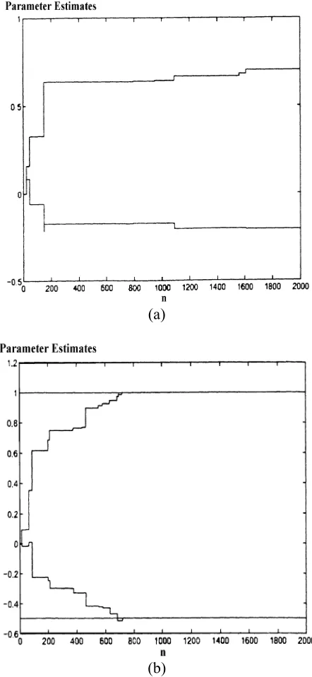
is assumed unknown. The results are shown in Figure 1 (See also the result of SM--SA OBE algorithm used in [13]).

Case 2. Time Invariant Parameter with

Multi Level Noise

In this case

v

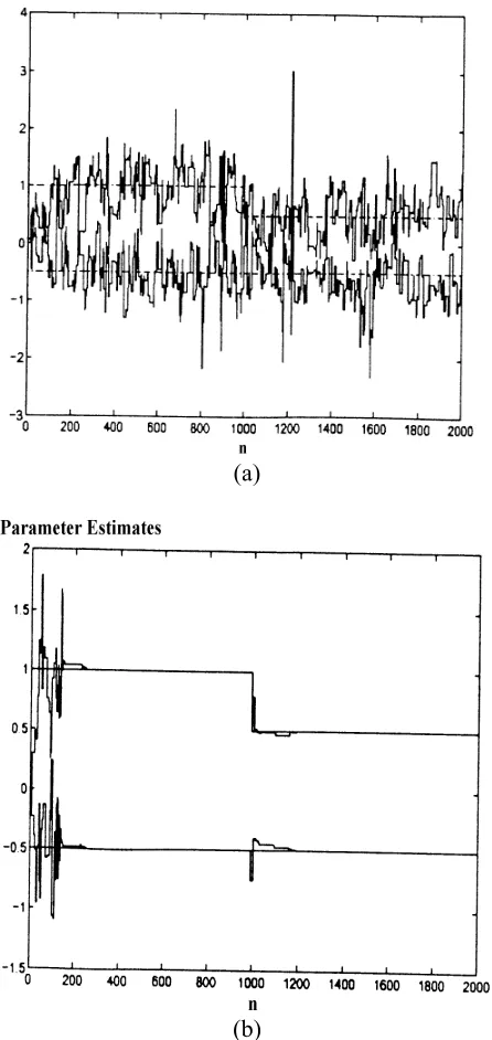
_n assumes values {-1,-2/3,-1/3,0,1/3,2/3,1} with equal probabilites. Other conditions are the same as case 1. The results are shown in Figure 2.

Case 3. Time Varying Model

The parameter

c

was changed by 50 % at one-thousandth sample, while

c

was kept constant at its nominal value. As before,

v

_n chooses values {-1,-2/3,-1/3,0,1/3,2/3,1} uniformly. The parameter estimates are plotted against the true values in Figure 3. The proposed algorithm also has remarkable performance for the case of under bounding.

bounding, MNLMS is unstable. Despite of all results, it is important to point out that MNLMS algorithm has remarkable performance when true

γ

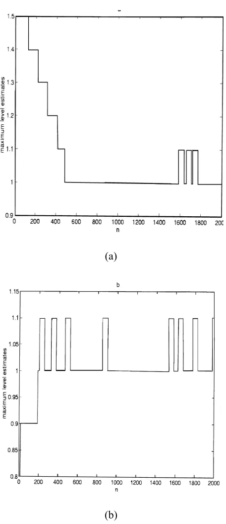
is available [12].

As mentioned in the end of section 2,

γ

_n finally

settles in the interval

[

γ∗−δ_,γ∗+δ

]

To illustrate this fact, Figure 5 shows the (a)

(b)

Figure 1. Parameter estimates for case 1 (a) MNLMS with

5

.

1

=

γ

and (b) proposed algorithm with

γ

=

1

.

5

, M = 50 and L = 2.

(a)

(b)

Figure 2. Parameter estimates for case 2 (a) MNLMS with

5

.

1

=

estimated values of

γ

∗

(

i

.

e

.

γ

_n

)

, calculated by ABE--MNLMS algorithm in the cases 3 and 4. In the cases 3 and 4 , the initial value of

γ

was

5

.

1

0

=

γ

and

γ

₀

=

0

.

8

respectively. Figure 5 (a

and b) shows that after n=500 (in case 3) and

200

=

n (in case 4) ABE--MNLMS algorithm has found its true value. Because of the value of L (L=2) that is small, there is not any underestimating after these time instants.

(a)

(b)

Figure 3. Parameter estimates for case 3 (a) MNLMS with

5 . 1

=

γ

and (b) proposed algorithm with

γ

=1.5, M = 50 and L=2.

(a)

(b)

Figure 4. Parameter estimates for case 4 (a) MNLMS with

8

.

=

CONCLUSION

A simple strategy to find the true maximum

level of noise has been derived. It is valid

for those measurement noises that reach

their maximum level in finite durations

with probability one. Simulation results

show that the tracking performance of this

algorithm in finding true maximum level

of noise is comparable to that of MNLMS

algorithm.

APPENDIX: PROOF OF THEOREM 1

Because

{ }

v_n is an MLS noise of order N, there are time instants

γ

≤

γ

∗in the sets of length N such that

( )

{

n iN,n i 1N 1

}

, i 0,1,2,K

k ,

vki =γ i∈ 0+ 0+ + − = ∗

(21) Suppose K is an integer multiple of N . Because_γ≤γ∗_{, the event}

1

,

,

1

,

,

=

_{0 0}

+

₀

+

−

<

+

u

n

n

n

n

K

v

_{n n}

γ

K

(22)

is covered by the event

( )

v

sign

( )

u

i

K

N

sign

_ki

≠

_ki

−

0

,

1

,

L

,

/

(23)

Hence

{

}

( )

( )

{

≠

=

}

<

ε

≤

−

+

+

=

γ

<

+

N

/

K

,

,

1

,

0

i

u

sign

v

sign

P

1

K

n

,

,

1

n

,

n

n

u

v

P

i i k k

0 0

0 n

n

L

L

(24) now suppose

{

v 0

}

p P

{

u 0

}

P p

i i 2 k k

1= > = > (25)

because

v

_n

and

u

_n

are independent for all

n

( )

( )

{

sign

v

≠

sign

u

i

=

0

,

1

,

,

K

/

N

}

=

P

i i k

k

L

(

p

₁

(

1

−

p

₂

)

+

p

₂

(

1

−

p

₁

)

)

K/N (26)

Hence under natural conditions that

(a)

(b)

42 - Vol. 15, No. 1, February 2002 IJE Transactions A: Basics

1

0

,

1

0

<

p

₁

<

<

p

₂

<

it is obvious that for the given there exists

M

₁ such that

(

)

(

)

(

−

+

−

)

1

<

ε

1 2 2

1

1

1

M

p

p

p

p

(27)

Choosing

M

=

M

₁

N

completes the proof.

REFERENCES

1. Fogel, E. and Huang, Y. F., “On the Value of Information in System Identification-Bounded Noise Case”,

Automatica, Vol. 20, (1982), 229-238.

2. Goodwin, G. C., Sin, K. S., “Adaptive Filtering, Prediction and Control”, Englewood Cliffs, NJ, Prentice-Hall, (1982).

3. Haykin, V., “Adaptive Filter Theory”, 3rd _{Ed., Englewood} Cliffs, NJ, Prentice-Hall, (1996).

4. Farhang-Borojeny, V., “Adaptive Filters: Theory and Applications”, John-Wiley and Sons, U.K., (1998).

5. Dasgupta, S. and Huang, Y. F., “Asymptotically Convergent Modified Recursive Least Squares with Data Dependent Updating and Forgetting Factor for Systems with Bounded Noise”, IEEE Trans. Inform. Theory, Vol. IT-33, No. 3, (May 1987), 383-392.

6. Hassibi, B., Sayed, A. H. and Kailath, T., “H∞ Optimality of the LMS Algorithm”, IEEE Trans. on Signal Processing, Vol. 44, No. 2, (Feb. 1996), 267-280. 7. Rao, A. K. and Huang, Y. F., “Tracking Characteristics of

an OBE Parameter Estimation Algorithm”, IEEE Trans. on Signal Processing, Vol. 41, No. 3, (March 1993), 1140-1148.

8. Deller, J. R., Nayeri, M. and Odeh, S. F., “Least-Square Identification with Error Bounds for Real-Time Signal Processing and Control”,Proceedings of the IEEE, Vol. 81, No. 6, (June 1993), 815-849.

9. Lin, V., Nayeri, V and Deller, J. R., “Automatic Bound Estimation: A Practical Development in Optimal Bounding Ellipsoid Processing”, IEEE Signal Processing Letters, Vol. 4, No. 8, (August 1997), 236-239.

10. Gollamudi, S, Nagaraj, S., Kapoor, S. and Huang, Y. F., “Set-Membership Filtering and a Set-Membership Normalized LMS Algorithm with an Adaptive Step Size”,

IEEE Signal Processing Letters, Vol. 5, No. 5, (May 1998), 111-114.

11. Durret, R., “Probability: Theory and Examples”, Wadsworth and Brooks/Cole Publishing Co., California, (1993).

12. Doost-Hoseini, A. M. and Shahtalebi, K., “NLMS Algorithm with Variable Step-Size Using Set-Membership Identification”, Submitted to Scientia Iranica.