A PARAMETRIC STUDY OF THE BEHAVIOR OF
GEOSYNTHETIC REINFORCED SOIL SLOPES
R. Qhaderi
Former postgraduate student of Geotechnical Engineering, IUT, Iran
M. Vafaeian and H. Hashemolhoseini
Lecturer, Isfahan University of Technology, Isfahan, Iran, [email protected], [email protected]
(Received: Nov. 2, 2004)
Abstract This paper presents the results of a number of computations using the 2D FEM to show the effects of significant variables on the behavior of geosynthetically reinforced earth slopes. The verification and reliability of the results are primarily examined through comparisons with experimental data available. The results seem to be quite acceptable and can be used with a high degree of reliability for predicting the relevant problems.
The main variables studied are soil properties, slope geometry, and the properties of reinforcement elements, while the safety factor, deformation components, effect of geotextile stiffness, the shape and location of the slip surface are the main unknowns sought.
Keywords Reinforced earth slope, Geosynthetic, Effective parameters, Safety factor
ه
ﺪﻴﻜﭼ
مﺮﻧﻪﻠﻴﺳوﻪﺑهﺪﺷ مﺎﺠﻧاتﺎﺒﺳﺎﺤﻣزاﻞﺻﺎﺣ ﺞﻳﺎﺘﻧ،ﻪﻟﺎﻘﻣﻦﻳارد رﺎﺘﻓرﻲﺳرﺮﺑصﻮﺼﺧرددوﺪﺤﻣياﺰﺟاراﺰﻓا
ﻲﻣﻪﺋاراﻚﻴﺘﺘﻨﺳﻮﺋژﻪﺑﺢﻠﺴﻣﻲﻛﺎﺧيﺎﻬﺒﻴﺷ دﻮﺷ
.
ﻪﺑﻪﺟﻮﺗﺎﺑ ﻞﻣاﻮﻋﺮﻴﺛﺄﺗﻞﻴﻠﺤﺗوﻲﺳرﺮﺑ،تﺎﺒﺳﺎﺤﻣﻦﻳاﻲﻠﺻافﺪﻫﻪﻜﻨﻳا
زاﺖﺳاترﺎﺒﻋﺎﻬﻠﻴﻠﺤﺗﻦﻳاردهﺪﺷبﺎﺨﺘﻧايﺎﻫﺮﻴﻐﺘﻣورﻦﻳازا،ﺖﺳاﺢﻠﺴﻣﻲﻛﺎﺧيﺎﻬﺒﻴﺷيﺎﻬﻴﻠﻜﺷﺮﮔدويراﺪﻳﺎﭘﺮﺑﺮﺛﺆﻣ
:
ﻪﺼﺨﺸﻣ ،كﺎﻜﻄﺻا ﺐﻳﺮﺿ و ﻲﮔﺪﻨﺒﺴﭼ ﻞﺜﻣ كﺎﺧ ﻲﺳﺪﻨﻬﻣ صاﻮﺧ ﻲﺘﺨﺳ ،عﺎﻔﺗرا و ﺐﻴﺷ ﻞﺜﻣ ﺰﻳﺮﻛﺎﺧ ﻲﺳﺪﻨﻫ يﺎﻫ
ﺋژ ﺎﻬﻧآﻪﻳوازوداﺪﻌﺗوﻞﻳﺎﺘﺴﻜﺗﻮ
.
ﻲﻣارتﺎﺒﺳﺎﺤﻣ ﻦﻳازاﻞﺻﺎﺣ ﺞﻳﺎﺘﻧ ﻦﻳاودادراﺮﻗهدﺎﻔﺘﺳا درﻮﻣﺢﻠﺴﻣيﺎﻬﺒﻴﺷرﺎﺘﻓرﻲﺑﺎﻳزرارد ﻲﻓﺎﻛنﺎﻨﻴﻤﻃاﺎﺑناﻮﺗ
ﻲﻘﻄﻨﻣوﺞﻳﺎﺘﻧﺖﺤﺻ ﺎﻬﻨﺗﻪﻧﻪﻛﺖﺳاﺖﻠﻋﻦﻳاﻪﺑ نﺎﻨﻴﻤﻃا زاﻲﻀﻌﺑ ﺎﺑﺞﻳﺎﺘﻧ ﻪﺴﻳﺎﻘﻣﻪﻠﻴﺳو ﻪﺑتﺎﺒﺳﺎﺤﻣشور ندﻮﺑ
ﺮﺠﺗتﺎﻋﻼﻃا ﺪﻴﺋﺎﺗولﺮﺘﻨﻛسﺮﺘﺳدردﻲﺑ
ددﺮﮔﻲﻣ ﺮﮕﻳﺪﻜﻳﺎﺑرﺎﮔزﺎﺳولﻮﺒﻗﻞﺑﺎﻗﻮﺤﻧﻪﺑتﺎﺒﺳﺎﺤﻣﺞﻳﺎﺘﻧﻪﻋﻮﻤﺠﻣﻪﻜﻠﺑ
ﻲﻣنﺎﺸﻧﻲﻘﻄﻨﻣﻲﮕﺘﺴﺒﻤﻫوﻲﻧاﻮﺨﻤﻫ ﺪﻫد
.
1. INTRODUCTION
Reinforced soil slope has been the subject of extensive research in the geotechnical field within the past 25 years, resulting in numerous publications on experimental results and theoretical analyses. Since H. Vidal (1969) proposed the mechanism and application of
reinforced earth, many aspects of this topic have been investigated. Moreover, at least seven international conferences have been so far held on the subject of the Geosynthetics.
both theoretical (better understanding) and practical (design procedure) viewpoints.
Generally speaking, studies of geosynthetically-reinforced soils can be categorized into analytical, experimental, or numerical types. According to Michalowski (1990), analytical studies of reinforced soil slopes can further be subdivided into three main groups. The first group is based on the conventional slice method, examples including studies by Reugger (1986) and Wright and Duncan (1991). The second, often called “structural method”, engages limit equilibrium analysis or the rotational equilibrium analysis. Among the studies based on this method, one can mention Schmertmann et al. (1987), Leshchinsky and Boedecker (1989), Jewell (1991, 96), and Michalowski (1990). The third group of analytical studies involves some kind of homogenization techniques such as those often employed in the analysis of composite materials, where the non-homogenous reinforced soil (soil and geotextile) is modeled as an anisotropic homogenous material. This method is also called “continuum method”. The approach by Sawicki and Lesniewska (1989) belongs to this group of studies.
During the last decade, outstanding experimental studies have been carried out on reinforced soil slopes. These studies, which are sometimes supplemented by numerical and analytical analyses, are performed either on real models (field dimensions) such as Chalaturnyk et al. (1990), or on reduced models by centrifugal apparatus such as Porbaha and Kobayashi (1998) and Zornberg et al (1998).
Nowadays, the numerical methods, and mainly finite element, have won universal acceptance in the geotechnical domain. Using appropriate constitutive models for soil and soil-structure interfaces and effective numerical techniques such as the arc length makes it possible to obtain a realistic model of reinforced soil slopes.
A review of about 13 previous experimental studies (from 1990 to 1998) have been reviewed by Zornberg and Arriaga (2000) in which the heights of slopes varied between 2.7m to 7.6 meters (with only one case of a slope with a height of 27.4 m).
Despite the rather numerous studies conducted on reinforced soil slopes, a number of important points still remain to be resolved. One such point
in need of clarification is the effects of geotextile stiffness and soil dilation on the stability of reinforced soil slopes and on the shape of shear band (failure surface). Using 2D finite element method, the present study aims to shed light on this issue. Here, a generic algorithm is used as a post-treatment tool to FEM for fitting an appropriate curve (circle or spiral) to failure surface.
2. BASIC VARIABLES FOR THE COMPUTATIONS
The Plaxis 2D program has been used to investigate a parametric study of reinforced cohesionless soil types. The type of reinforcement layers assumed in this study simulates the geo-synthetic sheets embedded within the soil layers while overturning on the top of each layer at the front edge of the slope (as the facing). The soil properties and the reinforcement design arrangements for the purposes of the present study have been chosen within the following ranges: Soil: φ = 28 to 43 degrees; ψ = 0 to 10 degrees; c= 10kPa; γ= 20 kN/m3
Slope geometry: Slope angle:
m
to
m
Height
to
73
,
6
18
45
=
=
θ
o oReinforcement design parameters:
EA (tensile stiffness): 150 to 10000 kN/m Number of Layers: 10 to 30
Length of reinforcement sheets: 2 to 12 m
Angle of reinforcement relative to the horizontal axis: 0 to 20o
The two dimensional mesh is generated by the automatic option composed of triangular elements including 15 nodes.
The output results computed by the program can be classified as follows:
1. Distribution of tensile stresses along each layer (kN/m);
2. Distribution of maximum tensile stress along the height of embankment;
3. Distribution of tensile strain on the vertical cross section;
4. Maximum amount and distribution of
5. Deformed mesh corresponding to the final stage of computation;
6. Shape and location of critical surface; and 7. Safety factor for each computation.
Both models of work-hardening and elastic Mohr-Coulomb were applied for the computations and the results were compared for any differences. Finally and based on the comparisons, the work hardening approach was selected. The selection is primarily based on the fact that the constitutive model which used in these analyses could not always reach a consistency and convergence. There are two technical points that should be mentioned for this matter:
1) In many elastic – plastic problem regarding the soil medium – rather than the slope stability- application of elastic –Mohr Coulomb in a finite element program does not face to an un convergency, while the computation procedure in slope stability may sometimes reach to a point of collapse at which the computation can not proceed further.
0 0.5 1 1.5 2 2.5
20 25 30 35 40 45
Friction Angle(degrees)
Sa
fe
ty
Fa
cto
r
Bishop Janbu Plaxis 2) The concept of safety factor in slope stability is
commonly based on the ratio of resisting agents to the disturbing agents ( either in terms of forces or the moments) along a predefined trial and assumed failure surface. On the other hand, within the F. E. M. programs for the soil medium the procedure of c-φ reduction is applied and the safety factor defined as the ratio of the actual existing values of these parameters to the reduced values which correspond to the collapse. The results of these two computations may be different specially for the reinforced soils but not for a simple soil medium.
3.RESULTS
It is universally known that both geometric and physico-mechanical properties of reinforced slopes are effective factors in slope behavior and stability. We first begin by comparing the FEM results with other analytical or experimental data; below are selected examples:
1) A comparison is made between the results obtained from Plaxis and those from the methods proposed by Janbu and Bishop (GEOSLOPE
downloaded from the Internet) for the safety factor values on a non-reinforced slope of 7.2m high with
3
/ 20 , 10 , 63
27to c= kPa = kN m
= γ
θ o o and the friction
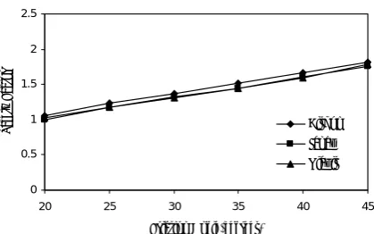
angle of 37o. This comparison is shown graphically in Figure 1 A similar comparison is presented in Figure 2 for the variations of friction angle from 20o to 45o for the same conditions and
the slope angle of 45o.
0 0.5 1 1.5 2 2.5
27 32 37 42 47 52 57 62 67
Slope Angle(degrees)
Saf
et
y F
act
or
Bishop Janbu Plaxis
Figure 1. Comparision of computed safety factor in three methods for the slopes with different slope angles.
Figure 2. Comparision of increasing the safety factor in three methods of computations for different values of
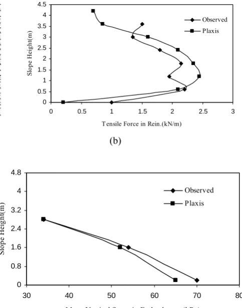
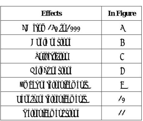
2) A simple example of actual reinforced slope (Fannin and Hermann,1990), as shown in Figure 3a, with a height of 4.8m, slope of 1H:2V, and reinforced with 8 large reinforcements (0.6m separation) with tensile stiffness of EA=150 kN/m is selected for the case study. The soil properties are as follows:
(a) (b)
Figure 3. (a) Cross section of an actual case of reinforced slope,
(b) Comparison between the computed and measured values of distribution of maximum tensile force in reinforcement layers of Fig. a;
(c)Comparison between the computed and measured values of mean vertical stresses along depth.
(c)
Friction angleφpl.st.= 38o and γ= 17 kN/m3.
The measured values of tensile forces in the reinforcement elements obtained from comparisons for the forces is illustrated in Figure 3b.
In Figure 3c, a comparison is made between the results obtained from Plaxis and the measured values for the vertical stress at levels 0.3, 1.5, and 2.7m from the base at a section of 1.5m from the slope face.
3) Another actual case is analyzed to compare the tensile forces within the reinforcement elements. Figure 4a shows the vertical section of a reinforced
step-wise slope wall in Italy (reported by Ghinelli and Sacchetti, 1998) with soil properties of
2 . 0 , 2 . 35 ,
0 , 33 , 4 .
18 = = = =
=
ϕ
ν
γ
o c Es MPa, H=15.5m, and a reinforcement tensile stiffness of 500 kN/m. Typical comparisons are shown in Figure 4b between the results of the present study by Plaxis and the results of F. E. M. by Ghinelli and Sacchetti (1998) for the tensile forces along the reinforcement layers of C, D, E, L and M as indicated in Figure 4a.
These examples promoted confidence about the correct use of Plaxis.
To evaluate the effect of each variable on the different aspects of slope behavior, several computations were carried out, and the results were categorized graphically in Figures 5 to 11 as described in Table 1.
0 0.5 1 1.5 2 2.5 3 3.5 4 4.5
0 0.5 1 1.5 2 2.5
Tensile Force in Rein.(kN/m)
Sl
ope
H
ei
ght
(m
)
3
Observed Plaxis
0 0.8 1.6 2.4 3.2 4 4.8
30 40 50 60 70 80
Mean Vertical Stress in Embankment(kPa)
Sl
op
e H
ei
ght
(m)
0 0.4 0.8 1.2 1.6 2
0 1 2 3 4
Distance from Slope Face(m)
5 R ei nf or cem en t S tr ai n( % )
Table 1. Discription of Figures
0 0.4 0.8 1.2 1.6 2
0 1 2 3 4 5
Distance from Slope Face(m)
R ein fo rc em en t S tr ain (% ) Plaxis F.E.M Plaxis F.E.M Field Data 0 0.4 0.8 1.2 1.6 2
0 1 2 3 4 5
Distance from Slope Face(m)
R ein fo rc em en t Str ain (% )
Effects In Figure
EA from 150 to 1000 5
Angle of slope 6
Soil friction 7
Height of slope 8
Number of reinforcements 9
Length of reinforcements 10
Reinforcement slope 11
Plaxis F.E.M Field Data 0 0.4 0.8 1.2 1.6 2
0 1 2 3 4 5
Distance from Slope Face(m)
R ei nf or cem en t S tr ai n( % ) Plaxis F.E.M Field Data 0 0.4 0.8 1.2 1.6 2
0 1 2 3 4 5
Distance from Slope Face(m)
R ein fo rc em en t S tr ain (% ) Plaxis F.E.M (C) (D) (E) (L) (M)
F.E.M.: (Ghinelli & Sacchetti,1998)Plaxis: (present study)
Figure 4 (a): Cross section of an actual stepped
reinforced soil slope,
In these Figures, the variations in tensile stress are shown in part (a) and the variations in safety factor are shown in part (b) while the values for displacements and shear strains are shown in parts (c) and (d), respectively.
An example of deformed mesh after failure and computed shear band is shown in Figures. 12 and 13, respectively.
4.DISCUSSION
The present results can be viewed from (at least) 3 aspects:
a) The effect of changing the properties of soil and/or reinforcement on the computed values of deformations, internal stresses and the overall calculated safety factor.
b) The location and the shape of failure surface; c) Comparisons and some complements for practical purposes.
a) The effect of variables on the computed values
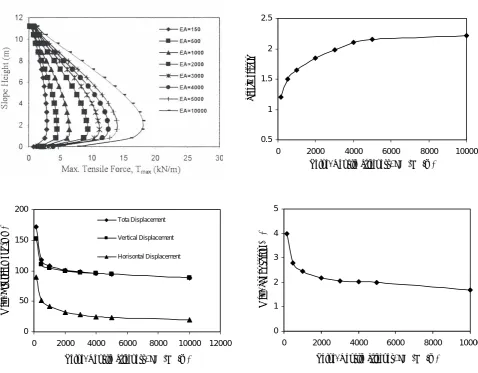
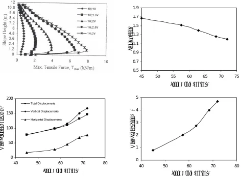
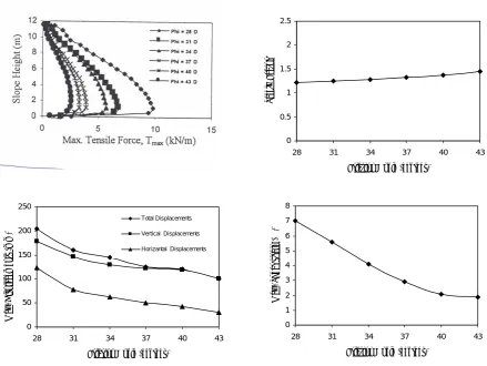
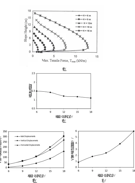
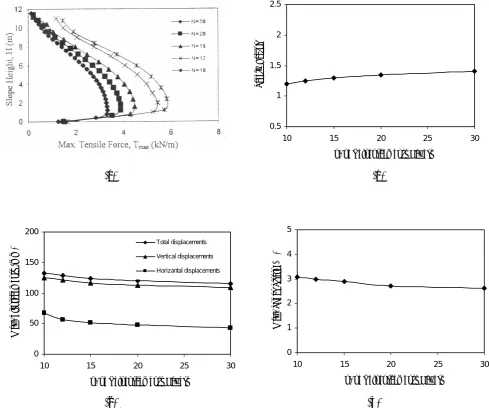
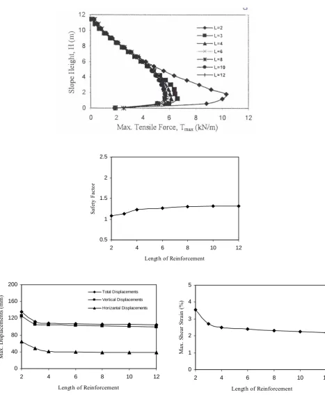
As expected, the slope angle and the slope height are the first and the main design requirements affecting stability or safety factor (Figures. 6b and 8b) and the deformation field (parts c and d in Figures. 6 and 8). The length of reinforcement elements by up to a length of 0.8H to 0.9H has some clear effects; but beyond that, higher lengths do not show any significant effect on the internal stability (Figure 10), though it should be checked for the pooling out safety. Increasing the stiffness of reinforcements (Figure 5b) and/or increasing the soil strength result in some higher safety factors (Figure 7b) and fewer deformations (Figures 5c and d, and 7c and d).
This type of response is quite predictable because of the interdependence of deformations and stiffness. Similar results have been reported by Han, Leshchisky and Shao (2002) for a computed case by FLAC in which they used the stiffness values from 200 to 4000 kN/m for cable elements in a slope with H=5 m, a slope angle of 45o,
composed of a cohesionless soil with E= 20 MPa and φ = 30o. The effect of increasing stiffness is
also clear on the maximum tensile stress along the reinforcement elements (Figure 5.a)
The present computations and graphs indicate that the values of strains corresponding to the least safety factor approximate rather large values, at least 2% (part d in Figures. 5 to 11). From this correlation, one can conclude that the failure of soil corresponds to the residual angle of friction (rather than the peak angle). Also the angle of dilatancy of sand does not show any (even small) effects on the results.
b) Shape of failure surface
As indicated in the literature, the geometrical shape of failure curve can be a matter of discussion in classical analytical computations and also in experimental observations.
The shape of failure surface cross section or the shear band can simulate both, with some approximations, circular and spiral curves in the first qualitative look, as illustrated in Figure 13. Nevertheless, analytical computations show that a circular curve can be better fixed with the view of obtained shear band.
Our computations indicate that the location of the shear band (zone) somehow depends on the overall stiffness of the slope–reinforcement system because when the reinforcement stiffness increases, this zone moves farther from the slope face. This finding can be seen by comparing parts a, b, and c in Figure 13.
In these computations, the shape of failure (shear band), shown by Plaxis, is sometimes quite clear while under some other conditions a wide band (or even a shadowy band) is obtained from which a sharp and deterministic curve can hardly be concluded. However, it is usually promising to pursue the place of plastic points of F.E. mesh (as in Figure 14) from which its limiting boundary can be the representing position of failure curve. Though the failure/shear band can be clearly traced on the vertical sections, the safety factor against the failure is not linearly dependent on the stiffness values of reinforcement (Figure 5b), on the friction angle of soil (Figure 7b), nor on reinforcement values (Figure 9b)
0.5 1 5 2 5
0 2000 4000 6000 8000 10000
Reinf. T ensile Stiffness, EA (KN/m)
Sa
fe
ty
fa
ct
or
1. 2.
0 1 2 3 4 5
0 2000 4000 6000 8000 10000
Reinf. T ensile Stiffnes, EA (KN/m)
M
ax
. S
he
ar s
tra
in
(%
)
0 50 100 150 200
0 2000 4000 6000 8000 10000 12000
Reinf. T ensile Stiffness, EA (KN/m)
M
ax.
D
is
pl
ac
em
ent
(
m
m)
Tota Displacement
Vertical Displacement
Horisontal Displacement
The computed results indicate that the location of failure zone depends to some extent upon the slope angle, length of reinforcements, and on their tensile stiffness. Increasing the slope angle will cause the failure zone to move deeper through the embankment. Also with increased stiffness, the failure bond moves deeper through inside and tends to occur within the non-reinforced part. Considering the above facts, deciding about the real geometrical shape of failure curve (whether circle or spiral) can always be a matter of uncertainty. Nevertheless, a number of mathematical tools presently exist that may be employed to show the comparative advantage of one assumption over another.
Figure 5. Computed effect of tensile stiffness of reinforcement elements (from 150 to 10000 kPa) on: (a) the values of maximum tensile forces ( Tmax, kN/m) and its distribution along the depth,
(b) the factor of safety,
(c) displacement and (d) Max, shaar strain
For our present purposes and in order to find a best and compatible curve for the failure shape computed by Plaxis, the following prerequisites are primarily mentioned.
0 1 2 3 4 5
40 50 60 70 80
Slope Angle (degrees)
M ax . S he ar s tra in (% ) 0.5 0.7 0.9 1.1 1.3 1.5 1.7 1.9
50 55 60 65 70 75
Slope Angle (degrees)
Sa fe ty Fa ct or 45 0 50 100 50 00
40 50 60 70 80
Slope Angle (degrees)
M ax. D is pl ac em ent s (m m ) 1 2 Total Displacements Vertical Displacements Horizantal Displacements
Figure 6. Computed effect of slope angle of wa l on the same variables as in figure 5.l
To find the best mathematically-fitted curve to the computed failure curve, a computer program of genetic algorithm is used. This program is compiled on the basis of C++ computations and
applied as the tool for finding the curve of best fitting based on stochastically non-linear optimization procedure ( Michalewich,1992). The optimization criterion for the curve is based on the minimizing statement:
{
}
∑
= − − − − n i c i c ii x x y y
R
1
2 2
2 ( ) ( )
where, n is the number of given points on the accepted curve considered, xi and yi are the
coordinates of the points, and xc, yc and Ri are
coordinates of the spiral center and its radius, respectively, as shown in Figure 15.
The representing formula for the spiral is )
tan . ( exp
. −
β
ϕ
=a R
where, R is constant for a circular curve.
The best-fitted curve is accepted by minimizing the sum of square of errors (MSE) as:
∑
= − + − = n i ii y y
x x n MSE 1 2 0 2
0 ) ( )
0 50 100 150 200 250
28 31 34 37 40 43
Fricrion Angle (degrees)
M
ax
. D
is
pl
acem
en
ts
(
m
m
)
Total Displacements Vertical Displacements Horizantal Displacements
0 1 2 3 4 5 6 7 8
28 31 34 37 40 43
Friction Angle (degrees)
M
ax
. S
he
ar s
tr
ai
n (%
)
0 0.5 1 1.5 2 2.5
28 31 34 37 40 43
Friction Angle (degrees)
Sa
fe
ty
F
ac
to
r
Figure 7. Computed effect of friction angle of soil on the same variables as in figure 5.
where, xi and yi are the coordinates of the points
corresponding to the sliding curve obtained from the present finite element method and x0 and y0
are the coordinates of the points of the fitted curve.
In Table 2, the computed values for MSE are shown for the assumed and computed cases for both spiral and circular curves for the 17 cases considered in the present study. Because these numbers are far smaller for the circular shape than for the spiral one, the circular curve is more acceptable.
Figures 16 and 17 illustrate examples of the
best-accepted curve for the computed failure curve and the best-fitted curves of spiral and circle shapes for which the values of MSE are shown in Table 2. Figure 15 shows two cases with different values of EA=150 and 5000 kN/m, and Figure 16 shows two cases with different values for different numbers of reinforcement layers (N= 10, 30) but for the same slope.
c) Some practical compliments
0.5 1 1.5 2 2.5
6 9 12 15 18
Slope Hei
(a)
ght (m)
Saf
et
y F
act
or
(b)
0 50 100 150 200 250 300 350
6 9 12 15 18
Slope Height (m)
M
ax.
D
is
pl
ac
em
ent
s
(m
m) total Displacements
Vertical Displacements
Horizantal Displacements
0 1 2 3 4 5 6
6 9 12 15 18
Slope Height (m)
M
ax
. S
he
ar s
tra
in
(%
)
(c) (d)
0.5 1 1.5 2 2.5
10 15 20 25 30
No. of Rein rcements Layers
Sa
fe
ty
Fa
ct
or
fo
0 50 100 150 200
10 15 20 25 30
No. of Reinforc ents Layers
M
ax.
di
spl
ac
eme
nt
s
(m
m
)
em
(a) (b)
0 1 2 3 4 5
10 15 20 25 30
No. of Reinforcements Layers
M
ax
. S
he
ar
St
ra
in
(%
)
Total displacements
Vertical displacements
Horizantal displacements
(c) (d)
Figure 9. Computed effect of the number of reinforcement layers on the same
variables as in figure 5
(Zornberg et al. 1998). Our computations showed that the best compromise that can be accepted is the one shown in Figure 18, which is almost a linear distribution with the maximum value near the base (see part a in Figures. 5 to 11). This type of distribution of maximum tensile forces along the height is in agreement with experimental data obtained (see Figure 3).
0.5 1 1.5 2 2.5
2 4 6 8 10 12
Length of Reinforcement
Sa
fe
ty
F
ac
to
r
0 40 80 120 160 200
2 4 6 8 10 12
Length of Reinforcement
M
ax.
D
is
pl
ac
em
ent
s
(m
m)
Total Displacements Vertical Displacements
Horizantal Displacements
0 1 2 3 4 5
2 4 6 8 10 12
Length of Reinforcement
M
ax
. S
he
ar
St
ra
in
(%
)
0.5 1 1.5 2 2.5
0 5 10 15 20
Slope of Reinforce.
(a)
Layers (deg)
Sa
fe
ty
Fa
ct
or
(b)
0 50 100 150 200
0 5 10 15 20
Slope of Reinforce. Layers (deg)
M
ax.
D
is
pl
ac
eme
nt
s
(m
m
)
Total Displacements
Vertical Displacements
Horizantal Displacements
0 0.5 1 1.5 2 2.5
0 5 10 15 20
Slope of Reinforce. Layers (deg)
M
ax
. S
he
ar S
tra
in
(%
)
(c ) (d)
Figure 12. An example of the deformed mesh of the vertical cross section of a reinforced slope.
Figure 13. The shape and position of the critical shear band as obtained from the present computations for
three cases of the reinforcement tensile stiffness: (a) 150 kN/m;
Figure 14. Location of plastic and tension points
determined by PLAXIS Figure 15. Geometrical feature for an assumed spiral or circle curve.
Tensile Force in Reinforcement
Figure 18. Comparison between different shapes of distribution of tensile forces in the reinforced layers along the height: (a) experimental; (b) analytical; and (c) present study.
5. CONCLUSIONS
From the results obtained in this study, the following can be concluded:
1) The shape of relative distribution of tensile force along the wall height is rather independent of the length of reinforcement layers, their tensile stiffness, their number, and their slope angle to the horizontal axis, and also independent of the height of slope and soil properties such as friction angle and dilatancy angle. The distribution of tensile force within reinforcements is shown in Figure 18a.
2) The position of the reinforcement layer on which maximum tensile force occurs is located at an elevation of 13 to 17 percent of the total height, and this position is rather independent of the above-mentioned variables. However, the location of maximum tensile force on the reinforcement is solely dependent on the slope angle of the wall, and this location moves upward with reduced slope angle.
3) Increasing tensile stiffness and length of reinforcement elements can result in increased safety factor of the slope and decreased
deformations and shear strains; however, these effects are limited to up to certain values after which they fail to show any significant effects. 4) Because the computed strains at the failure are not small, it is concluded that the mobilized friction angle of soil at the failure is the residual friction angle. Also, the dilatancy angle seems to have no obvious effects on the behavior of reinforced soil.
5) Within the reinforced slopes with reinforcing elements of axial stiffness below 1000 kN/m, the point of maximum shear strain on the failure surface is nearly located at the intersection of the vertical line through the edge of the slope and the slip surface.
6) The cross section of failure surface is fitted with a circular arc, though it is even possible to coincide with a curve of logarithmic spiral with lower accuracy.
6. ACKNOWLEDGEMENT Engineering (199?). The authors would like to express their gratitude to IUT for their permission to publish the results from the dissertation. We would also like to thank Mr. Ezzatollah Roustazadeh from the English Language Center, IUT, for her time editing the first draft of this paper.
The numerical and graphical results reported in this paper are due to R. Qaderi in his unpublished dissertation submitted to the Civil Engineering Department, Isfahan University of Technology, Iran, for the Degree of Masters in Civil
Table 2. Properties and model characteristics for finding the best fitting curve
Logarithmic spiral Circular
Model and Properties
x Y A MSE X Y R MSE
150 4.32 20.75 17 0.311 -9.21 19.66 20.92 0.08
1000 6.54 24.01 19.95 .426 -12.84 26.42 29.48 0.08
2000 7.22 28.47 23.95 .419 -12.27 27.25 29.95 0.05
3000 13.83 29.81 23.05 .48 -7.98 32.78 33.93 0.07
EA KN/m
5000 13.94 19.56 15 .535 -.93 22.30 23.15 0.16
10 4.62 26.87 22.8 .38 -12.39 24.2 26.42 0.07
15 2.72 32.58 30.37 .46 -13.98 24.6 27.8 0.09
N=
30 6.63 33.42 28.88 .38 -13.47 28.72 31.48 0.1
1V 10.22 29.17 23.44 .36 -9.23 28.47 29.94 0.05
2V 3.86 28.95 26.04 .4 -13.59 24.02 27.64 0.07
1H:
3V 1.23 37.2 35.88 .49 -13.65 22.92 26.05 0.12
6 1.88 17.06 15.12 .21 -8.04 14.48 16.28 0.05
12 4.44 26.87 22.8 .38 -12.39 24.21 26.43 0.07
H(m)
18 7.52 37.45 31.55 .504 -19.68 37.87 41.88 0.17
30 9.14 23.1 18.87 .38 -6.33 23.06 23.57 0.07
37 3.74 28.95 26.04 .4 -13.59 24.02 27.44 0.07
Φ(0)
6. REFERENCES
1. Chalaturnyk R. J., Scott J. D., Chan D. H.
K. and Rechards E.A. Stresses and deformations in reinforced soil slopes; Canadian Geotechnical Journal, Vol. 27, pp. 232- 244, 1990
2. Fannin R. J. and Hermann S., Performance
data for a sloped reinforced soil wall; Canadian Geotechnical Journal, Vol. 27, pp. 676 – 686, 1990
3. Ghinelli A. and Sacchetti M., Finite element
analysis of instrumented geogrid reinforced slope; Proc. of Int. Conf. on Geosynthetics, Vol. 2, pp. 649- 654,1998
4. Han J., Leshchinsky D. and Shao Y.,
Influence of tensile stiffness of geosynthetic reinforcements on performance of reinforced slopes. Proc. 7th International Conf. on
Geosynthetics, France, Delmas and Gourc (edit.), Vol. 1, 2002, pp. 197- 200
5. Ingold T. S., Reinforced Earth, 1982
6. Jewell R. A., Soil Reinforcement with
geotextiles CIRIA, Special Publcation 123, 1996
7. Jewell R.A., Revised design charts for steep
reinforced slopes, Reinforced Embankment, theory and Practice, pp. 1-30 Thomas Telford, London, 1991
8. Leshchinsky D., Design dilemma: Use peak or
residual strength of soil; Geotextiles and Geomembranes, Vol. 19, 2001, pp.111-125
9. Leshchinsky D. and Boedeker R.H.,
Geosynthetic reinforced soil structures, ASCE, J of Geotech. Eng., Vol. 115, No. 10, 1989, pp. 1459- 1478
10.Leshchinsky D., Stability of Geosynthetic
reinforced steep slopes, Slope Stability Engineering, 1999, pp. 49-66
11.Michalewich Z., Generic algorithm + data
structure = evolution programs , Springer – Verlag, Berlin, Heidelberg, 1992
12.Michalowski R.L., Stability of uniformly
reinforced slopes; ASCE, J. of Geotec. and
Geoenv. Eng. Vol. 123, No. 6, 1990, pp. 546- 556.
13.Plaxis Manual, Version 7.2 A.A. Balkema,
Netherlands, 1998
14.Porbaha A. and Kobayashi M., An
Investigation of Hazard in Reinforced Embankment, Geotechnical Hazards, 1998,
pp. 251-258
15.Qhaderii R. Study of stability of
geo-synthetically reinforced slope by application of finite element program of Plaxis 2D., M.Sc. Thesis, Soil Mechanics and Found. Eng. Group, Civil Engineering Department of IUT, Iran, 2003
16.Reugger R., Geotextile reinforced soil
structure, Proc. Third Int. Conf. on Geotextile, Vienna, Austria, 1986, pp. 453-654
17.Sawicki A. and Lesniewska D., Limit
Analysis of Cohesive Slopes Reinforced with Geotextiles, Computers and Geotechnics, Vol.
7, No. 1, 1989, pp. 53-66
18.Schmertmann G. R., Chourey-Curties V. E.,
Johnson R. D. and Bonapart R. Design Charts for geogrid-reinforced soil slopes Proc.
Geosynthetics, Industrial Fabrics Assn., Int. St.
Paul, Minn., Vol. 1, 1987, pp. 108-120
19.Vidal H. (1969a), The principles of reinforced
earth. Highway Res. Rec., No. 282, pp. 1-16
20.Wright S. G. and Duncan J. M., Limit
Equilibrium Stability Analysis for Reinforced slopes, Transp. Res. 1330, Transp. Res. Board,
Washington, 1991, pp. 40-46
21.Zornberg J.G., Sitar n. and Mitchel J.K.,
Limit equilibrium as basis for design of geosynthetic reinforced slopes, ASCE, J. of Geotech. & Geoenv. Eng., Vol. 124, No. 8, 1998, pp. 684- 698
22.Zorenberg J. G. and Arriaga F., Reinforced
Soil Design: Integration of digital image analysis, numerical modeling and limit equilibrium, Technical Report, Colorado