DOI 10.1007/s11538-006-9181-x
ORIGINAL ARTICLE
Evaluation of Experiments for Estimation of Dynamical
Crop Model Parameters
Ilya Ioslovich
a,∗, Per-Olof Gutman
aaFaculty of Civil and Environmental Engineering, Technion-Israel Institute of Technology, Haifa 32000, Israel
Received: 3 April 2006 / Accepted: 2 November 2006 / Published online: 15 February 2007 C
Society for Mathematical Biology 2007
Abstract Planned experiments are usually expected to provide maximal benefits within limited costs. However, there are known difficulties in optimal design of experiments. They are related to the case when only limited number of parameters could be estimated, because available experiments are noninformative. The useful method for this case is considered based on the dominant parameters selection procedure (DPS). The methodology is illustrated here with data from five planned experiments related to the NICOLET lettuce growth model. The maximal number and the list of estimated parameters are determined while the conditional number of the information Fisher matrix (modified E-criterion) is kept below a given upper constraint.
Keywords Sensitivity analysis·Planning of experiments·Nicolet model
1. Introduction
Lettuce is becoming an important component of human food and lettuce consump-tion continuously increases all over the world. A stable and high-quality lettuce product supply is required throughout the year for industrial purposes as well as for home kitchens. However, concerning the health hazard associated with high level of nitrate in leafy vegetables, the EC issued a directive (194/97), defining maximum levels for nitrate in fresh vegetables, including lettuce and spinach. Low light levels in winter often make it difficult for growers to meet the required stan-dard. The history of mathematical modeling of lettuce is at least 25 years old. Proper modeling of the lettuce growth is based on a set of previously revealed biological phenomena. In particular, several basic researches (e.g., Bolm-Zastra
The conference version of this paper has been presented at the 16th IFAC World Congress, July 4–8, 2005, Prague, Czech Republic.
∗Corresponding author.
and Lampe, 1985; Drews et al., 1995) have shown that the nitrate concentration in lettuce is negatively correlated with the level of soluble carbohydrates. More specifically, increased carbohydrate concentrations, associated with photosynthe-sis at higher light levels, led to lower nitrate concentrations in lettuce. The dy-namic model NICOLET (Seginer et al.,1998) assumed that the pool size of non-structural carbohydrates (including soluble sugars) is determined by the balance between source activity (supply by photosynthesis) and sink activity (demand by maintenance and growth). The plant is assumed to posses a regulation mechanism that adjusts the nitrate concentration in its cells to the fluctuating carbohydrate level, in order to meet the turgor requirement. Any change in growing conditions that leads to an increase of source activity relative to the sink activity, should re-sult in accumulation of soluble carbohydrates, thus diminishing the need for ni-trate as a cellular osmoticum. Hence, the scope for controlling nini-trate accumu-lation in vegetables could be considerably larger than previously thought. Opti-mal control policy including reduction of N-supply was presented inIoslovich and Seginer(2002) andDe Graaf et al.(2004). Modeling of crop quality is a relatively new field, in which there is considerable potential for progress. Development of a generic method to accurately control an important quality aspect of greenhouse vegetables, i.e., internal nitrate concentration, constitutes a significant contribution to scientific advancement. The model-based control of dynamical processes often strongly depends on the reliability of the involved models. The costly experiments are carried out in order to provide data for the proper calibration of the models, i.e., to estimate its parameters. The known approach to optimize this process is an optimal design of experiments, by finding appropriate inputs, seeKalaba et al. (1973),Fedorov(1972),Goodwin and Payne(1977),Munack and Posten(1989), and others. Clearly, this method is demonstrated inKalaba et al.(1973), using a one-dimensional dynamical system. The criterion maximized is an integral of the difference between the square of the parameter sensitivity (information content) and the integrated cost of the control during experiment. The model of the dynam-ical system is
dx
dt = f (x,y,p,t), (1)
where x is a state variable, u is the control input, p is the system parameter, and t is the time. The sensitivity of the state variable x to parameter p along the trajectory is S(t)= ∂x
∂p,and
dS dt =
∂f
∂xS+
∂f
∂p. (2)
should be constrained so that it varies within the feasible region and also its cost will be limited. The objective function is taken as
I=
T
t0
(S2−gu2) dt, (3)
where g is a weighting coefficient, and the first term is an one-dimensional simpli-fication for the Fisher information matrix. The multidimensional cases are consid-ered e.g. inVereecken and Van Impe(1998) andVan Impe and Versyck(2000). A very smart technique and interesting results are shown inKeesman and Stigter (2002) andStigter and Keesman(2004). In these works, some scalar functions of the Fisher information matrix (usually a modified E-criterion: ratio of the maximal to the minimal eigenvalue) are used as an indication of good performance of the experiment. The performance has to be understood in the sense of the ability to es-timate the model parameters. This approach, however, leads to a multidimensional optimal control problem, where the control inputs to the system must be found to-gether with state variables and their sensitivities to all parameters. Let us say there are n state variables and m parameters. The dimensionality of the problem then will be n+n×m.In the papers mentioned earlier, the problems are related to biotechnology and the optimal control problems are of low dimensionality and the Fisher matrix is nonsingular. This is not the case for the range of biological and environmental models, seeKlepper(1971), and many crop growth models. Cali-bration of crop growth models is a very cost and time consuming operation and it is highly desirable to know in advance what information will be possible to ex-tract from the limited set of available experiments. More definitely the question is: which parameters will it be possible to estimate. Often, not all model param-eters can be successively identified and a try and error procedure is used to find a reasonable subset of identifiable parameters. One also must notice that there arise essential difficulties in the optimal experiment design when Fisher matrix is singular. When a subset of parameters can be found such that the Fisher matrix is nonsingular, then the method of the optimal design of the experiment can be proceeded for this subspace. It will be shown later how the Dominant Parameter Selection (DPS) procedure,Ioslovich et al.(2004), can solve this problem and the evaluation of experiments for the lettuce growth model NICOLET will be demon-strated.
2. DPS procedure
x(t) with nominal values of the system parameters p and given control inputs u.
The column vector Skj(ti)=∂Y∂kp(ti)
j is the sensitivity vector of the model output Yk to parameter pj at the moments ti when the measurements are planned. These sensitivities can be found by solving the correspondent linearized time-dependent equations along the nominal trajectory of the dynamical system (model), or can be found numerically. The components of the vector are multiplied by the weights
ωi k, which can be chosen in a different way. Often the time-related index i can be omitted and weightsωkcan be used instead. This is a usual substitution for unknown inverse covariance matrix of the measured errors, see Munack and Posten(1989) andMunack(1991). The column vector Sj will then be a notation for concatenation of the vectors ωkS
j
k. The matrix S is defined as a horizontal concatenation of the column vectors Sj. The Fisher matrix can be written as
F=S∗S. (4)
The rank of the Fisher matrix indicates if the matrix is degenerate and the condition number (ratio of maximal to the minimal eigenvalue) will indicate if it is ill conditioned. This means that some of parameters are correlated or almost correlated. Then, the optimization search for the best fit over the set of parameters will follow the ridge (submanifold) where the different values of parameters will give the same or almost the same values of the objective. This can occur when sensitivities are linearly dependent, e.g., only a combination of parameters can be extracted from the calibration in the conditions of the experiment. According to DPS, a subset of parameters for the model calibration must be chosen from the most sensitive (dominant) and independent parameters. From the eigenvalues of the Fisher matrix, the dimensionality of this subspace can be found as follows. First, an upper thresholdα1 for condition number of the submatrix is selected. Next, the normalized Fisher matrix is formed according to the rule
Snj = S
j
(Sj)(Sj)
(5) Fn=Sn∗Sn,
correlation. The correspondent submatrix of the Fisher matrix must be formed and the eigenvalues are computed. If the condition number of the submatrix is too large according to the established threshold (i.e., cond> α1), then the least sensi-tive parameter is excluded and the most sensisensi-tive among remaining parameters is included, unless the list of sensitive parameters will be empty. In this way, the max-imal parameter subset is found with an upper constraint on the conditional number of the Fisher submatrix. For crop growth models, a logarithmic Least-Square Esti-mation is often used which provides some normalization for data of different ages of the exponentially growing crop. In this case, the relative sensitivities
skj= pj Yk
∂Yk
∂pj
(6)
can be used for the same purpose. The vector sjis determined in the same way (as concatenation of the weighted vectors), as the vector Sj, and matrix s is formed as the horizontal concatenation of the vectors of the column vectors sj. The product
s∗s will be the modified Fisher matrix Fm. The advantage of the relative sensi-tivity is that it is dimensionless. The normalized matrix also must be calculated in the same way for modified Fisher matrix and the same selection procedures must hold. We shall demonstrate this approach with the NICOLET lettuce growth model and evaluation of the available set of experiments. This procedure was also used for calibration of different dynamical models, seeIoslovich et al.(2002),De Graaf et al.(2004),Bortolin et al.(2002),Linker and Johnson-Rutzke(2004), etc.
3. The NICOLET model-short description
NICOLET lettuce growth model (Seginer et al.,1998,1999) is based on the com-plementary properties of nitrate and carbon in the vacuoles. The calibration of the model was considered inVan Straten et al.(1999). Several studies with lettuce produced clear negative linear correlations between sugar and nitrate in the cell sap. The model is used for the lettuce growth optimization and quality control (in terms of the nitrate content). Several basic assumptions have been made. The vol-ume occupied by the vacuoles is a fixed fraction of the total volvol-ume of the plant. The nitrogen-to-carbon ratio in the structure is also fixed. The ratio in the vacuoles is variable and constrained by the need to maintain a constant turgor pressure. Respiration and growth are assumed to depend on temperature. The nitrate flow into the vacuoles is calculated from the demand to support growth and to maintain turgor. The model has two state variables, the carbon content of the vacuoles and the carbon content of the structure, MCvand MCs, respectively. Other components, like nitrate content in the vacuoles and in the structure, can be expressed in terms of these state variables. The state equations of the model are
dMCv
dt = FCav−FCm−FCg−FCvs,
(7) dMCs
where FCavis the photosynthetically generated carbon flux (subscript C) from the atmosphere (a) to the vacuoles (v); FCm and FCg are the maintenance (m) and growth (g) respiration fluxes; and FCvsis the flux of carbon from the vacuoles into the structure (s), namely growth. The photosynthesis flux, FCav, and the growth flux, FCvs, are modeled as products of three factors: (i) The uninhibited flux for a closed-canopy crop, (ii) a measure of light interception (surface cover) by the canopy, and (iii) an inhibition function. Thus,
FCav= p{I,CCa}f{MCs}hp{Cv},
p{I,CCa} =
IσCCa
I+σCCa,
(8)
FCvs=g{T}f{MCshg{},
g{T} =νe{T},
where p{I,CCa}is the gross-photosynthesis rate, determined by light, I, and by at-mospheric (or greenhouse) CO2concentration, CCa; g{T}is the potential growth rate, which is a function of temperature, T; f{MCs}is a measure of light intercep-tion,
f{MCs} =1−exp{−a MCs}, (9)
which approaches one as the canopy closes; and hp{Cv}and hg{Cv}are, respec-tively, dimensionless photosynthesis and growth inhibition functions, which in the uninhibited state are equal to 1. hpdepends on parameters bpand sp, and hg de-pends on parameters bg and sg, respectively. The first approaches zero for high values of the normalized carbon (sugar) concentration in the vacuoles,Cv, while the second approaches zero for low values ofCv. The respiration fluxes were for-mulated as
FCm = f{MCs}e{T}, e{T} =k exp{c(T−T∗)}
(10)
FCg=θFCvs,
whereθ is a constant fraction. The nitrate concentration in the vacuoles, CNv, can be obtained from the carbon concentration, CCv, as
Cv +Nv=1,
Cv =
βCCCv
v
, (11)
CN= β NCNv
v ,
state variables MCvand MCsvia
MNv=
λv
βN
MCs−
βC
βN
MCv
(12)
MNs=rNsMCs,
whereλis the permanent water volume associated with one unit of structural car-bon; rNsis the N to C permanent ratio in the structure. A nitrogen balance of the vacuoles has the form,
dMNv
dt =FNrv−rNsFCvs, (13)
where dMNv
dt is the rate of change of the nitrate-N content of the vacuoles, FNrvis the uptake of nitrate from the rhizosphere. If growth is limited by nitrate supply, then uptake is equal to supply and FNrvrepresents the rate of supply. From Eqs. (12) and (13), one can easily get
βNMNv+βCMCv=vVv (14)
and
dMNv
dt =
λv
βN dMCs
dt −
βC
βN dMCv
dt , (15)
where Vvis the volume of the vacuoles per unit ground area. It is now possible to derive an expression for the rate of growth, FCvs, in terms of the limiting supply rate of nitrate, FNrv(and other quantities). Using Eq. (15) to substitute fordMNv
dt in Eq. (13) and then substituting for time derivatives of MCvand MCsfrom Eqs. (8), an expression for FCvs in terms of the other fluxes is obtained for the N-limiting case
FCvs=
βNFNrv+βC(FCav−FCm)
vλ+βC(1+θ)+βNrNs
. (16)
Using Eq. (16) completes the modification required for the nitrate-limited growth. One way to determine the missing initial condition is to assume that since the plants are initially small and the environment constant, growth is balanced and exponential (EG). The composition of seedlings growing under such conditions is only a function of the environment and hence invariant with time. Therefore, the ratio is assumed for the initial data
MCv
MCs
= dMCv
4. Evaluation of the available experiments
A set of the available experiments for estimation of parameters of the NICOLET model is considered. In these experiments, the normal and the extreme climate conditions were expected to be maintained in the greenhouse. The extreme exper-iments were associated with: low level of the source inputs, namely light and CO2, and low sink demand associated with low level of Nitrate supply and low inside air temperature. All the conditions are expected to remain permanent (no day–night changes) during the period of 1 month. Daily measurements of the four outputs were planned. All the experiments were planned in such a way that the Equilib-rium Growth (EG) conditions in all cases will be maintained. Following values of climate inputs were taken as the normal (i.e., summer conditions in Israel):
Light, I=20 mol [PAP] m−2d−1
Nitrate supply, FNrv=0.65 mol [N] m−2d−1 Inside air temperature, T=24,47◦C
Inside CO2concentration, CO2=0.0353 mol [C] m−3
The inside temperature was chosen to get hg=0.5 from the EG Eq. (17). Cor-responding values of thev and values of the inhibition functions for the four extreme experiments are shown as follows.
Source stress conditions:
Low CO2, CCa=0.005 mol [C] m−3, hg=0.5,
Cv=bg,
Low light, I =8.006 mol [PAP] m−2d−1,
hg=0.5, Cv=bg
Sink stress conditions:
Low temperature, T=12.62◦C,hp=0.5,
Cv=bp,
Low Nitrate, FNrv=0.0157 mol [N] m−2d−1,
hp=0.5, Cv=bp
Four model outputs were planned to be measured each day during 1-month pe-riod for these experiments. They are:
FM[g m−2]: fresh mass, DM[g m−2]: dry mass,
NO3[mg [NO3] kg−1[FM]]: Nitrate,
Nr[g [N] g−1[DM]]: reduced Nitrogen.
Altogether 15 model parameters were analyzed for possible selection into the Fisher matrix subset for the estimation. These parameters are related to photosyn-thesis (, σ), respiration and growth (θ, k, ν, c), photosynthesis and growth (a),
experiments will permit to identify some parameters related to the photosynthesis and growth and/or growth inhibition, and the low sink growth experiments will permit to identify some parameters related to the photosynthesis inhibition and/or N to C ratio in the structure.
The nominal values of parameters were taken as follows: Photosynthesis:
=0.07 mol[C]/mol[PAP]; σ =1.4×10⁻³m/s Respiration and growth:θ=0.3; ν=13.6
k=0.147(10−6mol[C]/(m2[ground] s);
c=0.06931/K
Photosynthesis and growth:
a=1.7 m2/mol[C]
Internal relationships:
βN=6.0 kPa/(mol[N]/m3);
βC=0.61 kPa/(mol[C]/m3);
λ=0.833×10⁻³m3/mol[C]
Inhibition functions:
bp=0.8; sp=10; bg=0.2; sg=10
Nitrogen to Carbon ratio in the structure:
rNs=0.08 g[N] g−1[C]
The previous parameters were included in the sensitivity analysis and evaluation of the experiments. In addition, the following values were used:
Conversion:
η=0.030 kg[DM]/mol[C]
Initial condition (fresh mass):
Wi
F=0.0093 kg/m2
Arbitrarily fixed: T∗=20◦C
The sensitivity analysis was done numerically. Relative sensitivities were calcu-lated (one point per each day) for each of four outputs along the trajectory of each planned experiment with nominal values of parameters. The results of the analysis
Table 1 Normal conditions
k rNs
Table 2 Source-limited growth
a λ βN rNs
Low light 1 4 (38.2) 3 (5.3) 2 (1.4)
Low CO2 1 3 (5.7) 2 (1.1)
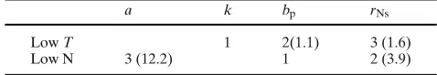
of availability of parameters estimation are presented for these five experiments separately and also for all experiments together (as a combined data set) in the Tables 1–4. The selection procedure DPS follows its description in Section 2. The thresholdsα1=0.95, α2=40 were used in the DPS procedure. In Tables 1–4, for the correspondent treatments, the selected parameters are shown with their num-ber in the order by decreasing sorting set of the relative sensitivities and the corre-spondent condition number (in brackets) for the Fisher submatrices where these parameters are selected. In the case when the parameter is the first in the order, the condition number is not indicated (because then the dimension of the submatrix matrix is 1).
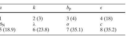
For all experiments considered together as a union source of the modeled data, the results of the DPS procedure are presented in Table 4. The eight selected pa-rameters are shown.
One can see that in Table 4, almost the union of the parameters selected for the separate treatments is presented. Generally, one can see that different parameters are selected for the source-limited experiments and for the sink-limited experi-ments. It looks natural that in both source-limited experiments with low light and low CO2parameter, βNis selected. As far as in this case, the nitrate concentra-tion prevails in the vacuole. However, it is also expected that parameter bpfrom the photosynthesis inhibition function hpis a significant one when the sink stress occurs as a result of the input reductions in the case of low temperature and also for low nitrate experiments. Parameter rNsis an important one for the constant N to C ratio in the structure and thus it affects the outputs in both type of experi-ments. From the first look, it is not clear whyis selected in the experiment with low light andσ is not selected in the experiment with low CO2. However, it can be understood by consideration of the relative sensitivities of the photosynthesis
[image:10.441.106.345.556.597.2]p{·}in respect to these parameters. The relative sensitivity of photosynthesis with respect tois inversely proportional to I and the correspondent relative sensitivity in respect toσis inversely proportional to CCa. For the used normal conditions, the productI is fivefold less than the productσCCa. The same ratio exists between their relative sensitivities in the experiments with low I and low CCa, respectively. The combination of multiple experiments together provides more variability in conditions and thus permits to select more parameters for the estimation. One can see that the most wide set of parameters (eight parameters) can be extracted from consideration of all treatments together.
Table 3 Sink-limited growth
a k bp rNs
Low T 1 2(1.1) 3 (1.6)
Table 4 All treatments
a k bp
1 2 (3) 3 (4) 4 (18)
βN λ σ c
5 (18.9) 6 (23.8) 7 (35.1) 8 (35.2)
5. Conclusions
An analysis and evaluation of several planned experiments for parameters estima-tion has been presented. This can be considered as a preliminary and necessary step for optimal design of experiments that overcome difficulty related to the Fisher matrix singularity. A simple preliminary procedure DPS has been used. It gives a suggestion of choosing parameters for estimation as a result of the future experiment. The procedure was demonstrated with a set of possible experiments for estimation of parameters of the NICOLET model. It was shown that the type of experiment (sink- or source-limited growth) corresponds to the selection of the parameters. A combination of different experiments is more effective rather than consideration of the separate treatments.
Acknowledgements
The authors are grateful to Professor I. Seginer for useful notes and suggestions.
References
Bortolin, G., Gutman, P.-O., Nilsson, B., 2002. Modelling of out-of-plant hygroinstabililty of multi-ply paper board. In: Proceedings of the MTNS Workshop. University of Notre Dame, South Bend, IN, August 12–16, pp. 303–325.
De Graaf, S.C., Stigter, J.D., van Straten, G., Belayert, P., 2004. Enhanced information extraction from output sensitivity analysis for practical calibration of dynamical models illustrated on a greenhouse climate model. European Project FAIR CT98-4362 (NICOLET), Final report. Draper, N.R., Smith, H., 1981. Applied Regression Analysis. Wiley, New York.
Fedorov, V.V., 1972. Theory of Optimal Experiments (Translated from Russian end edited by W.J. Studden and E.M. Klimko), Probability and mathematical statistics, No. 12, Academic Press, New York, London, pp. 292.
Goodwin, G., Payne, R.L., 1977. Dynamic System Identification: Experiment Design and Data Analysis. Academic, New York.
Ioslovich, I., Seginer, I., 2002. Acceptable nitrate concentration of greenhouse lettuce: Two opti-mal control policies. Biosyst. Eng. 83(2), 199–215.
Ioslovich, I., Seginer, I., Baskin, A., 2002. Fitting the NICOLET lettuce growth model to plant-spacing experimental data. Biosyst. Eng. 83(3), 361–371.
Ioslovich, I., Seginer, I., Gutman, P.-O., 2004. Dominant parameter selection in the marginally identifiable case. Math. Comput. Simul. (MATCOM) 65, 127–136.
Kalaba, R.E., Springarn, K., 1973. Optimal inputs and sensitivities for parameter estimation. J. Optim. Theor. Appl. 11(1), 56–67.
Keesman, K.J., Stigter, J.D., 2002. Optimal parameter sensitivity control for the estimation of kinetic parameters in bioreactors. Math. Biosci. 179, 95–111.
Linker, R., Johnson-Rutzke, C., 2004. Modeling the effect of abrupt changes in nitrogen availabil-ity on lettuce growth, root-shoot partitioning and nitrate concentration. Agric. Syst. 86(2), 166–189.
Ljung, L., 1999. System Identification. Theory for the User. Prentice-Hall, Englewood Cliffs, NJ. Munack, A., 1991. Criteria to optimize measurements for model identification. In: Rehm, H.-J.,
Reed, G. (Eds.), Biotechnology. VCH, Weinheim, FRG, p. 680.
Munack, A., Posten, C., 1989. Design of optimal dynamical experiments for parameter estimation. In: Proceedings of the American Control Conference, ACC89, Pittsburgh, PA, pp. 2011– 2016.
Nelles, O., 2001. Nonlinear Systen Identification. Springer-Verlag, Berlin.
Seginer, I., Van Straten, G., Buwalda, F., 1998. Nitrate concentration in greenhouse lettuce: A modelling study. Acta Hortic. 456, 189–197.
Seginer, I., Van Straten, G., Buwalda, F., 1999. Lettuce growth limited by nitrate supply. Acta Hortic. 507, 141–148.
Stigter, J.D., Keesman, K.J., 2004. Optimal parametric sensitivity control of a fed-batch reactor. Automatica 40(8), 1459–1464.
Van Impe, J.F., Versyck, K.J.E., 2000. Solving dual optimization problems in identification and performance of fed-batch bioreactors. In: Preprints, International Conference on Mod-elling and Control in Agriculture, Horticulture and Post-Harvesting (Agricontrol 2000), Wageningen, The Netherlands, pp. 25–36.
Van Straten, G., Lopez Cruz, I., Seginer, I., Buwalda, F., 1999. Calibration and sensitivity analysis of a dynamic model for control of nitrate in lettuce. Acta Hortic. 507, 149–156.