www.ann-geophys.net/30/1515/2012/ doi:10.5194/angeo-30-1515-2012
© Author(s) 2012. CC Attribution 3.0 License.
Annales
Geophysicae
Collisionless reconnection: magnetic field line interaction
R. A. Treumann1,2, W. Baumjohann3, and W. D. Gonzalez4
1Department of Geophysics and Environmental Sciences, Munich University, Munich, Germany 2Department of Physics and Astronomy, Dartmouth College, Hanover NH 03755, USA
3Space Research Institute, Austrian Academy of Sciences, Graz, Austria
4Divis˜ao de Geof´ısica Espacial, Instituto Nacional de Pesquisas Espaciais, S˜ao Jos´e dos Campos, S˜ao Paulo, Brazil Correspondence to: R. A. Treumann ([email protected])
Received: 16 February 2012 – Revised: 14 July 2012 – Accepted: 11 September 2012 – Published: 9 October 2012
Abstract. Magnetic field lines are quantum objects carrying one quantum80=2πh/e¯ of magnetic flux and have finite radiusλm. Here we argue that they possess a very specific dynamical interaction. Parallel field lines reject each other. When confined to a certain area they form two-dimensional lattices of hexagonal structure. We estimate the filling factor of such an area. Anti-parallel field lines, on the other hand, at-tract each other. We identify the physical mechanism as being due to the action of the gauge potential field, which we de-termine quantum mechanically for two parallel and two anti-parallel field lines. The distortion of the quantum electrody-namic vacuum causes a cloud of virtual pairs. We calculate the virtual pair production rate from quantum electrodynam-ics and estimate the virtual pair cloud density, pair current and Lorentz force density acting on the field lines via the pair cloud. These properties of field line dynamics become im-portant in collisionless reconnection, consistently explaining why and how reconnection can spontaneously set on in the field-free centre of a current sheet below the electron-inertial scale.
Keywords. Space plasma physics (Magnetic reconnection)
1 Introduction
In a recent communication (Treumann et al., 2011) we devel-oped the microscopic concept of magnetic field lines as be-ing central to the problem of collisionless reconnection. This concept was based on the well-established quantum mechan-ical principle (Aharonov and Bohm, 1959; Landau, 1930) that in a magnetic field B the magnetic flux is quantised. We demonstrated that, on the elementary level of two field lines (or elementary flux tubes) with each one carrying one
quantum 80=2πh/e¯ of flux and with the magnetic fields in the flux tubes being of opposite direction, merging of the flux tubes annihilates a total of precisely two flux quanta, 18=4πh/e. There is nothing mysterious about this fact of¯ merging. It is a purely classical process. No quantum elec-trodynamics has to be called for. Once the flux tubes do get into contact over the anti-parallel length`k along the field
lines, they will necessarily spontaneously merge and annihi-late. For a magnetic field of strengthB, the radius of a field line is given by
λm= p
80/π B. (1)
This allowed an estimate of released power in a single ele-mentary merging event toP0∼4π Bh`¯ k/µ0e, being propor-tional to the magnetic field strength and the parallel contact length. We also demonstrated that, because of the finite field line cross-sectionπ λ2m, the annihilation process and the re-leased power are sensitive functions of the angle under which the field lines get into contact.
2 Implications for collisionless reconnection
The micro-scale field-line merging and flux quantum annihi-lation processes raise the non-trivial question of how mag-netic field lines can be brought into mutual contact. This question is part of the more general problem of the mech-anism of interaction between magnetic field lines.
the volume of ion-inertial radiusr < λi=c/ωi surrounding the reconnectionX-point (ωi is the ion plasma frequency). Ions become non-magnetic, decouple from the magnetic field
B, follow their inertia and, in addition, become accelerated in any electric field that would be present, e.g. the cross-tail convection electric field, in the case of the magneto-spheric tail. No convincing mechanism has been identified yet that would be capable of causing reconnection on the scale of the “ion diffusion region”. Electrons remain mag-netised, freeze the magnetic field to their cyclotron orbits and transport it convectively across the “ion diffusion re-gion”. In this way they cause Hall currents (cf., e.g. Son-nerup, 1979). The physics of reconnection is thereby de-ferred to the electron-inertial scale “electron diffusion” re-gionr < λe=c/ωearound theXpoint (withωethe electron plasma frequency) where the electrons become non-magnetic as well. Since they cease to transport the magnetic field in this region, the question raised is how the magnetic field can be transported further into the very centre of the current sheet in order to get into close contact with the oppositely directed field and magnetic flux and reconnect.
2.1 Field line transport
The present communication is devoted to the investigation of this question as a pre-requisite to the understanding of macro-scale reconnection in view of its geophysical appli-cation. Details are given in the Appendix. The obvious triviality of this question relates to the fact that, under non-driven reconnection conditions, there is no known classical process which acts to transport the magnetic field inward into the current sheet in order to bring the oppositely directed field lines into mutual contact. This is immediately transpar-ent. Under driven conditions, in the presence of convective field transport into the current sheet, the field will accumu-late at the electron inertial scale boundary until the magnetic pressure becomes large enough to push some magnetic field lines further inward (Baumjohann et al., 2010). This accumu-lation has so far not been accounted for in any of the Harris current sheet models used in initiating reconnection. Macro-scale consequences of such driving have been investigated by Pritchett (2005) with the help of sophisticated and carefully performed numerical simulations.
In the absence of driving, to which most reconnection models and simulations refer, simulations usually circum-vent the transport problem by either imposing, globally or lo-cally, an artificial resistivity – or any other kind of dissipative mechanism – in the current sheet (implicitly referring to the respective original models of Parker, 1958; Petschek, 1964) or simply impose brute force seedX-points in order to initiate reconnection (the method described in Zeiler et al., 2002, and widely used by the PIC community). All these attempts do not explain the onset of reconnection as a fundamental phys-ical process. They, instead, properly account for the various macro-scale effects of reconnection which may occur under
various conditions when reconnection has already set on and
continues to take place.1This approach is well justified un-der the assumption that some unspecified mechanism gener-ates the seedX points. Such mechanisms have been based on magnetic fluctuations or the action of some electromag-netic instability (e.g. whistlers, kielectromag-netic Alfv´en waves, or the Weibel modes proposed in Treumann et al., 2010).
In the Appendix, starting from the field-line microscopic concept (Treumann et al., 2011), we investigate the sub-microscale mechanism of the interaction of elementary flux tubes for the two cases of parallel and anti-parallel mag-netic field lines. This mechanism requires reference to quan-tum electrodynamics. There we show that on the scales of non-magnetic electrons below the electron cyclotron radius r < rce∼
p
T⊥/B2the field lines carrying flux elements
or-ganise in a lattice of hexagonal pattern (see Fig. B2) with lattice constantd. This lattice is “frozen” to the electron cy-clotron orbit.
When the electrons approach the boundary of the electron inertial region near the centre of the current sheet and de-magnetise (see Fig. 1), their gyroradius increases to become larger than the electron inertial scale. At this instant, the lat-tice of magnetic field lines explosively dews, the field lines become released, and the lattice structure dissolves (undergo-ing phase transition similar to two-dimensional lattice melt-ing in solid state physics, cf., e.g. Huang, 1987).
From now on, the field line dynamics is determined by the repulsive forces between the parallel field lines and stresses which result from a possible local bending of field lines. For straight field lines we ignore the latter. Then the released field lines from the dissolved lattice are pushed inward into the field-free region of the current sheet by the repulsive forces. Here, they meet field lines of opposite direction, which en-tered the neutral current layer from the other side of the cur-rent by the same mechanism. The oppositely directed ele-mentary flux tubes now experience attractive forces, become accelerated toward each other in order to approach quickly and, when coming into close contact, collide and annihilate the flux quanta stored in them over a certain parallel length `k.
2.2 Transition to reconnection
Since many a number of field lines are added to the neu-tral layer, it is clear that a large number of field lines par-ticipate in merging and annihilation, adding up to macro-scale reconnection-flux tubes and causing the different in-ferred macro-scale effects reconnection offers under the var-ious external plasma conditions. In this way, the dynamical interaction of field lines provides the wanted consistent pic-ture of spontaneous onset of reconnection.
1For a conservative review, see Biskamp (2000). A recent
λ
2eJ
[image:3.595.89.508.64.325.2]
Fig. 1. Three meso-scale flux tubes encountering the electron inertial region at the centre of a (symmetric) current layer which separates two plasmas with anti-parallel fields. The (blue) field above the currentJ points into the plane, the (red) field below the current points out of the plane. Above and below the electron inertial layer the field is frozen to the electrons (not shown) forming a lattice structure. When entering the electron inertial region, the lattices break off and dissolve as the fields become released from the frozen-in state. Under the action of the repulsive gauge fields they seek to achieve larger distances whereby entering the central region. Meeting field lines of different polarity from the other side, they feel attractive gauge forces (indicated by green lines), approach each other and annihilate (yellow stars). The distribution of merging centres is statistical. Merged field lines relax and join up to produce macro-scale reconnection effects: jets etc.
In view of a possible observational confirmation of the sub-microscale merging of field lines and cause of re-connection, one is currently bound to spacecraft measure-ments which, unfortunately, cannot resolve any of the sub-microscales under question. Indirect evidence is the only way of experimentally checking the reality of our theory. This ev-idence may be given by observation of wave2 or radiation processes in the three different stages of merging in the chain of reconnection: initial single field line merging, followed by inclusion of dielectric effects, mass loading by electrons, and finally the already known macroscopic stage of mass loading by ions. The first two interesting stages are sub-microscale (Treumann et al., 2011). They occur when the curvature ra-diusrc of the merged field lines is shorter than the Debye length
λm< rc< λD. (2) As long as this holds, the merged and strongly kinked field line relaxes like in vacuum. This field line relaxation is iden-2Wave observations related to reconnection are sparse, low
fre-quency examples can be found in LaBelle and Treumann (1988), Baumjohann et al. (1989, 1990), Treumann et al. (1990) and Bale et al. (2002).
tified as free-space electromagnetic radiation of frequency fem, i.e. high-frequency electromagnetic radiation in vac-uum. Since it is expected that in reconnection in a current layer very many field lines merge, this will cause an elec-tromagnetic radiation spectrum in a fairly broad frequency range:
c/λD< fem< c/λm. (3) Rewriting this expression yields:
c βeλe
< fem<
102−103(BnT)
1
2 GHz, (4)
where the lower limit is determined by the velocity ratioβe= ve/cand the electron inertial scale lengthλe=c/ωe, andBnT is in nT. This can also be written as:
30ωe √
Te
< fem<
102−103(BnT)
1
2 GHz, (5)
Once, however, the curvature radius reaches the Debye length, dispersion of the electromagnetic waves changes due to modification of the dielectric properties, and the emit-ted radiation becomes cut off at the plasma frequency. The short wavelength, high-frequency radiation escapes from the reconnection site and enters the surrounding magnetised plasma, where its polarisation properties come into play. One may expect that the original emission would be non-polarised, i.e. emission is isotropic. Hence, in the magnetised plasma it will split to equal amounts into right and left-hand polarisations. This produces a mixture of high frequency L-O-mode and R-X-mode radiation.
So far it is not yet clear whether or not the initial radi-ation will indeed be isotropic. The degree of polarisradi-ation will depend on the merging mechanism of single field lines, which will to some degree also be affected by the torsion of the magnetic field line flux tube (which might be substantial because of the finite radius of the field lines), which deter-mines the polarisation of the radiation. Possibly the torsions, and thus the polarisations, are different on both sides of the current sheet, however, which would make a distinction for emission of radiation on either side of the reconnection site. The related questions are open to investigation.
At later stages, when the curvature radius exceeds the elec-tron inertial scale, the elecelec-trons become magnetised, and the fluctuations propagate in the whistler or Z-mode bands. Ob-servation of the form of radiation in relation to reconnection signals the sub-microscopic mechanism of field line merging. Reconnection itself is identified to be a sub-microscale phenomenon. It can be understood on the basis of the quan-tum concept of magnetic field lines and their interaction via their external gauge fields. Macroscopic reconnection then becomes an intrinsically three-dimensional phenomenon: the interaction of many merging (sub-microscale) anti-parallel field lines forming large numbers of reconnection specks. As a by-product, it also makes clear why spontaneous recon-nection is a statistical phenomenon which occurs in small patches resembling turbulent (or patchy) reconnection.
3 Conclusions
The present communication just resolves the problem of field line transport in the electron inertial region inside the current sheet under non-driven conditions. This is just a pre-requisite of the problems related to macro-scale reconnection. It sug-gests, however, that the ultimate understanding of the micro-physics of reconnection probably requires inclusion of mag-netic field line dynamics, i.e. the dynamics of magmag-netic flux quanta80. Merging and annihilation of such flux quanta is possible only by direct contact of anti-parallel sections of the field-line flux tubes.
This can be understood as being due to the interaction of field lines via their external gauge fields. Most of the space between field lines is void of any magnetic fields. The
inter-action in question can be repulsive or attractive. Repulsive interaction is found between parallel field lines and, if the magnetic field is confined to a certain spatial volume of finite area, causes a hexagonal lattice structure of the field. On the other hand, attractive interaction occurs between anti-parallel field lines. The combination of repulsion and attraction is the main reason why field lines can enter into the centre of a neutral current layer separating plasmas of opposite magnetic field direction, and is thus the basic cause of sub-microscale field line merging. In principle, it solves the problem of re-connection on the quantum level.
The discussion given in this communication clarifies the main physics with only a limited amount of reference to the full quantum electrodynamics instrumentation of magnetic field line dynamics. The gauge field external to a magnetic field line is capable of creating a small number of virtual electron-positron pairs which live on the “borrowed” time of quantum mechanical uncertainty. These pairs contribute to a weak though finite Lorentz force between elementary magnetic flux tubes, which for parallel field lines is repulsive and for anti-parallel field lines is attractive. This is the basic quantum physics of field line interaction.
Macroscopically observed reconnection effects come to birth when many a number of field lines become involved, merge, relax and become ultimately mass loaded. The result-ing chain of processes for two anti-parallel field lines has been described in an earlier paper (Treumann et al., 2011). Involvement of a very large number of merging field lines in some particular location requires a proper statistical ap-proach.
The macroscopic effects of reconnection will be rather different for different external conditions in the interacting plasmas and different parameter settings. However, the sub-microscale cause of merging and reconnection is quite gen-eral and independent of the macro-scale settings. It involves attracting magnetic field lines of opposite direction in or-der to penetrate into the centre of the neutral current layer and for coming into mutual contact, a problem which has been treated in the present communication. Under collision-less conditions, this kind of attraction is independent of any external macro-scale differences.
Appendix A
Field line concept
The flux can be positive or negative, depending on the di-rection of the magnetic field±B. Each magnetic field line being a flux tube of radius
λm= r
80
π B, (A1)
the “magnetic length” of Landau (1930). He inferred this length from the quantum-mechanical motion of an electron in a homogeneous magnetic field, finding that the perpendic-ular electron energy⊥= ¯hωce(n+12)would be quantised, with ωce=eB/me the non-relativistic4 electron cyclotron frequency,meelectron rest mass, andn=0,1, .... One easily recognises that the “magnetic length” corresponds to the gy-roradius of an electron in the lowest Landau level (LLL), i.e. the gyroradius of an electron of very low energy. Its coinci-dence with the field-line radius implies that the smallest
gyro-cross section an electron could possess in a given magnetic
fieldB, is the cross-section of a magnetic flux tube of one quantum of magnetic flux80, i.e. one field-line. Under space conditions near Earth, with magnetic fields of the order of 1.B.105nT, this energy is very small, 10−13.LLL. 10−8eV. At electron temperatures of the order of 1 eV.Te in space, the low Landau levels will be empty. Thermal Lan-dau levels (TLL) occupied by thermal electrons have quan-tum numbers centred aroundnTLL&1010and forming ther-mal continua.
Hence, one distinguishes between the respective low en-ergy and thermal enen-ergy regimes. The former is the strongly coupled regime of the Quantum Hall Effect. Strong coupling means that electrons and magnetic field quanta are closely tied via the Laughlin wave function of the electrons (Laugh-lin, 1983) which extends the Landau solution to many elec-trons. In this low-energy regime, electrons are forced to oc-cupy Landau levels. Electrons in the lowest Landau level plus flux quanta form a fluid consisting of quasi-Fermions or “composite electrons” with effective chargeq=e/3 and, for particular magnetic field strengths, lead to quantisation of the Hall resistance.
In the thermal regime, electrons become independent of flux quanta. Their dynamic scales, being of the order of the electron gyroradiusrceλm, grossly exceed the field-line scale, and the coupling between electrons and field lines be-comes weak. On the other hand, on scales< rce below the electron gyroradius the dynamics of magnetic flux quanta is independent of the presence of electrons. In this regime, large numbersNce of flux quanta (field lines) are adiabati-cally confined to the electron gyroradius and undergo mutual short-range interaction. This number is proportional to the ratio of the gyration-to-field line cross-sections:
Nce∼ π rce2 π λ2 m
= E⊥ ¯ hωce
, (A2)
4Having in mind application to space problems like
reconnec-tion at the magnetopause and in the geomagnetic tail, we do not attempt to treat the relativistic case here.
whereE⊥=p2⊥/2me, and p⊥ is the perpendicular electron
momentum. This number is not completely conserved, how-ever, during one electron gyration. Gyration takes time1t∼ 2π/ωceduring which a field line may escape to the environ-ment. The uncertainty ofNce≈1E⊥/¯hωceis obtained from the uncertainty relation1E⊥1t∼hto amount to only
1Nce∼1. (A3)
Hence, during one electron gyration, the number of the many adiabatically trapped field lines in the electron gyra-tion cross-secgyra-tion either lost or added to the frozen-in mag-netic flux is of the order1Nce=O(1)only. Under frozen-in conditions, this number forms an electron gyration flux tube and is convected together with the electron across the plasma. The frozen-in magnetic field lines are parallel to each other within mutual inclination angles 0≤θ <12π, being unable to undergo merging (Treumann et al., 2011). The angular de-viations may be caused by magnetic fluctuations of various origin and are of no interest for the following. During con-vection of the plasma, allNcefrozen-in field lines are carried across the plasma. Referring to the reconnection site, they are carried toward the centre of the current sheet in the process of reconnection when the electrons cross the “ion diffusion region” but have not yet entered the electron inertial region in the centre of the reconnection site.
Appendix B
Field line topology and lattice
The first interesting point is that the value of the above num-ber Nce is slightly over-estimated by the naive assumption of dense packing of field lines. Quantisation of flux distorts the continuous distribution of magnetic fields. Parallel field lines (flux tubes) exert repulsive forces on each other, seek-ing to expand into space and separate as distant as possible from neighboring field lines. This is due to the Lorentz force-like interaction between the flux tubes and is well-known from classical field-line patterns like, for instance, those of dipolar or quadrupolar fields. Classically, the Lorentz force on a magnetic flux tube with field strengthB1, exerted by a neighbouring flux tube of field strength B2, is given by F12= −∇(B1·B2)/2µ0+(B1· ∇)B2/µ0. The second term accounts for the stresses produced by bending or twisting the flux tubes. In the absence of any bending only the first term survives. Clearly, sinceB∼1/rα, withα >0 some power,
parallel field lines are subject to positive (repulsive), anti-parallel field lines to negative (attractive) forces.
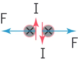
This is illustrated in Fig. B1 for the case of two closely spaced field lines which point into the plane. Putting one test-electron in LLL state on the circumference R=r/λm=1 of each field line, the electrons gyrate clockwise, each pro-ducing a circular line currentI = −I0δ(R−1), with I0= ephω¯ ce/meλ2m∼10−21
p
× ×
I
I
F
[image:6.595.313.543.64.210.2]F
Fig. B1. Repulsive interaction between two closely spaced parallel field lines pointing into the plane and each carrying one electron in its lowest Landau level, LLL. Electron gyration is clockwise and confined to the circumference of the field line (red circles), produc-ing anti-parallel currentsIred arrows). These currents give rise to repulsive forcesF (blue arrows).
currents, indicated by the red arrows, cause repulsive Lorentz forces between the parallel field lines of strengths per unit length F ∝2µ0I02/r∼10
−48√ω
ce/λ3mR. The forces be-come attractive for two anti-parallel field lines where the cur-rents flow parallel to each other. However, the field lines are located in vacuum, and no LLL electrons are available. In this case the interaction is not obvious, as we will discuss in detail below in Appendix C and D.
For parallel field lines carrying one flux quantum only, and being confined to a spatial cross-section like the gyration-cross section of the electron, this subtle interaction causes a very particular arrangement of field-lines. Rejecting and keeping themselves at distancesdλmfrom each other, in a homogeneous magnetic field, they create a lattice of field lines consisting of hexagonal elements, with one field line in the centre surrounded by six field lines in the corners of the hexagon; every field line spanning its own hexagon with the space between the field lines being void of magnetic fields. This is shown in Fig. B2 and differs from the continuous field distribution in classical physics on the macro-scale. On the sub-microscale, the quantisation of the magnetic flux causes a lattice structure of the magnetic field.
The homogeneous field-line filling factor follows from comparing the cross sections of field line and hexagon. The latter consists of six triangles of side lengthsd0=d+2 where d0is the centre-to-centre distance between two neighbouring field lines, andd >1 is the external vertical distance between the field lines, both in units ofλm. The field-line free surface of the hexagon (hexagon surfaceSH=3
√
3d02λ2m/2 minus the surfacesSfl=3π λ2m contributed by the field line in the centre and those in the corners) becomes:
Sempty=Sfl "
2 √
3 d 2
2 +1 !
−1 #
. (B1)
d
Fig. B2. Repulsive interaction between confined parallel field lines generates a hexagonal lattice composed of elementary flux tubes and magnetic field lines, each carrying just one flux quantum80= 2πh/e¯ . Every corner of a single hexagon is occupied by a field line, as shown on the right (small black circles of radiusλm). If field lines are trapped, like in the frozen-in concept, then the number of field lines is roughly six times the number of hexagons which can be fitted into the cross section of an electron cyclotron orbit. The red circles indicate the repulsive quasi-potential barriers which build up around each field line as a result of the presence of the mutually interacting gauge fields (see below). The circular shape of these barriers holds approximately for nearest neighbor interactions only. The gauge fields of each field line are confined to their own circle. The open triangular regions between the red circular barriers are close to being free of any gauge fields.
This yields the field-line filling factor:
qfl= Sfl SH
=√ 2π
3(d+2)2. (B2)
The distanced between the field lines is determined by the repulsive force between the parallel field lines and is not easy to determine without any knowledge about the force between the field lines and the size of the volume of the plasma to which it is confined. We delay this question to the discussion in the next section.
Assuming that the field lines are confined to the electron gyro-cross section, the number of field lines in this cross sec-tion is determined dividing it by the surface of the hexagon, finding that an electron cyclotron-cross section contains
Nflce∼√2π Nce
3(d+2)2 (B3)
[image:6.595.98.225.66.165.2]cross-section must be larger by the factor
B
hBi ∼ √
3 2π(d+2)
2. (B4)
Unfortunately, there is no obvious and simple independent determination of the “lattice constant”d becaused is a dy-namical quantity which adjusts itself to Lorentz force equi-librium between the entire ensemble of field line flux tubes in the volume. Assuming thatB/hBi ∼103yields a lattice con-stant ofd∼15. IfB/hBi ∼10 this value reduces to d∼3 only. One may conclude that generally, the field concentrated in one field line will be strong and the cross section small.
In aβ∼1 plasma one has for the average magnetic field hBi2∼2µ0NeTeobtaining for the magnetic field of one field lineB∼√3µ0NeTe/2(d+2)2. This will hold approximately in the “ion diffusion region” until one enters the electron in-ertial range.
Appendix C
Field-line interaction
Classically there is no answer to the question of how the force is transmitted across the field-free space between the field lines. In the absence of LLL electrons, no field exists outside the field lines except for the gauge fieldA= ∇3which does not directly contribute to any magnetic field. It is, in fact, the gauge field which takes care of the absence of magnetic fields outside the field line, keeping external space clean of magnetic fields. To use a common term: Field lines have no
hair.
We note in passing that the definition of the magnetic field through the flux element80and vector potentialA
B= A 2π λm
= 80 π λ2 m
(C1) implies that the magnetic vector potentialAof a magnetic field line is related to the magnetic field strength as:
A √
B =
r 80 4π =
r ¯ h
2e. (C2)
The right hand side of this expression is a constant, showing that the ratio on the left is quantised.
C1 Gauge field geometry
Even though it is intuitive, the classical argument of the Lorentz force given before does not apply, at least not in the conventional form. From the fact that, for a single isolated field line, ∇3 has only an azimuthal component (see, e.g. Aharonov and Bohm, 1959; Treumann et al., 2011) with3 being proportional to the azimuthal angleθgiven by 3(θ )=80
2πθ= ¯ h
eθ (C3)
0
1’ 2’
3’ 4’ 5’ 6’ 7’ 8’ 9’
1
2
3 4
17’
16’
15’
[image:7.595.311.544.62.246.2]14’ 6 5 7
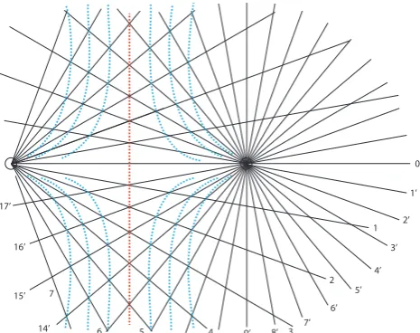
Fig. C1. Superposition of the equi-gauge potential lines3=const of two parallel magnetic field lines (elementary flux tubes carrying one flux quantum8o=2πh/e¯ ). Equi-gauge potentials are exactly radial, emanating from their mother field line. The field lines are shown in their cross sections and point out of the plane. They are separated in space by some distanced. The equi-gauge potentials are clockwise numbered consecutively with the equi-gauge poten-tials of the right field line indicated by primes on the numbers. Since potentials add the superposition of the equi-potentials, generating the dashed repulsive potential pattern in the space between the field lines, this indicates that the interaction between a pair of parallel field lines is subject to repulsion.
one concludes that the gauge field3 is constant in the ra-dial direction – meaning that radii are gauge-field “equi-potentials” as shown by the black radials emanating from the two circles representing field lines in Fig. C1.
Analytically one adds up the two gauge fields 31(θ ) of field line 1 and32(θ0)of field line 2. The anglesθ, θ0 are measured in the respective proper frames of field line 1 and 2, the origin of the latter being displaced along the x-axis by the distancedfrom the origin of the former. The total gauge field is a potential field which is additive, being the sum 3=31(θ )±32(θ0)=
80 2π θ±θ
0
, (C4)
where the+-sign refers to parallel field lines, the−-sign to anti-parallel field lines. The angleθ0is to be transformed into the proper frame of field line 1 such thatθ0(θ, r;d)becomes a function of distanced (in unitsλm) between the field lines, angleθ(in radians), and radiusr(also in unitsλm). The angle θ0maps to an angleθvia the relation
tanθ0= Rsinθ
Rcosθ−1, R= r
d, (C5)
which when used in the above sum yields the expression: 3(θ, R)=80
2π
θ∓tan−1
Rsinθ 1−Rcosθ
for the quantum-mechanically correct total gauge field in the space external to the two field lines. TheRandθdependence of the second term in the brackets in Eq. (C6) destroys the strictly radial pattern of equi-gauge potentials, with the main region of interest beingR <1.
The gauge field equi-potentials are obtained by holding ex-pression (C6) constant. This yields the equi-gauge equation: R(θ,3)˜ = tan θ− ˜3
cosθhtan θ− ˜3±tanθi
(C7)
˜ 3≡2π
80
3=const. (C8)
Varying3˜ and calculatingR(θ,3)˜ for each fixed value of3˜ produces a pattern of equi-gauge potentials which now has become dependent of radiusR. This dependence is enforced by the mere presence of another field line at distancer=d. Clearly, if the distance between the field linesdris large, i.e.R1, this pattern degenerates to the original radial pat-tern of one isolated field line, as is seen from Eq. (C6). Again, the±signs apply to parallel and anti-parallel field lines. C2 Equi-gauge potential construction
It is easy to geometrically construct the shape of the equi-gauge potentials by superposition. This has been done schematically in Figs. C1 and C2 for the two respective cases of parallel and anti-parallel field lines; here we plot the equi-gauge potentials for two (stretched) field lines in the perpen-dicular plane under the condition that each field line would be isolated in space and no other field lines would be present. In the parallel case the solitary patterns of both field lines are of course identical, being numbered clockwise. In the anti-parallel case they are numbered in opposite order (i.e. the anti-parallel field line radials are numbered anti-clockwise). Superposing the two gauge fields produces the dashed curves in these figures.
The important and intuitive observation is that for parallel field lines half way between the two field lines, the superpo-sition of the gauge fields creates a separation barrier in the gauge potential, which forces the superimposed gauge field equi-potential field lines to deviate up to 90◦from their radial directions. This enforces a pronounced radial dependence of the gauge equi-potential field according to Eq. (C7). The pat-tern is similar to the equi-potentials produced by two elec-tric charges of equal sign causing repulsion of the charges. Extrapolating to our case of two interacting parallel field lines, we may conclude that it is the repulsive action of the
gauge fields between the two parallel magnetic flux tubes
which keeps the parallel field lines on distance. It is this ac-tion which is responsible for the generaac-tion of the hexagonal structural lattice order of the field shown in Fig. B2.
Figure C2 shows the plot of the equi-gauge potentials for the case when the magnetic fields are anti-parallel. In this case the left flux tube points out of the drawing plane, the
18’
17’
16’
15’
14’ 13’ 12’ 11’
1
2
3 4
1’
2’
3’
4’ 5
[image:8.595.311.545.62.243.2]6 7
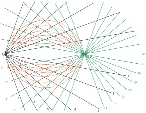
Fig. C2. Superposition of the equi-gauge potential lines3=const of two anti-parallel magnetic field lines. The field lines are shown in their cross sections with the left field line pointing out of the plane and the right field line pointing into the plane being spatially separated by some distanced. The equi-gauge potentials are again clockwise numbered consecutively. Because of the opposite direc-tion of the field in the right field line the primed equi-gauge poten-tials are numbered anti-clockwise. Addition of the equi-gauge po-tentials yields the dashed equi-gauge superposition pattern of con-nected equi-gauge potentials in the region between the field lines. Such a pattern indicates attraction between the oppositely directed field lines mediated by the gauge fields.
right tube points into the plane. By having turned the right flux tube by 180◦into the plane, the rotational sense and thus
the counting of the equi-gauge potentials is reversed. When superimposed with the equi-gauge potentials of the left flux tube, the picture of the dashed lines is obtained in this case. It is obvious that now the equi-gauge potentials of the two flux-tubes connect and an attractive gauge-potential structure is obtained.
C3 Numerous field lines
Equation (C4) can be generalised to many field lines by sum-ming over their respective anglesθi0and accounting for their varying distances from the origindi. Choosing one reference field line as the origin and the distanced0to one of its neigh-bours as direction of the x-axis, one has:
tanθi0= Rsin θ +αi
Rcos θ+αi−Di
, R= r d0
, Di= di d0
>0. (C9) Here, 0≤αi≤2πis the angle the direction ofdimakes with the direction of the x-axis, i.e. the direction ofd0. The nor-malised total gauge potential field is the sum over all contri-butions from theifield lines:
˜
3(θ, R)=X i
(
θ∓tan−1 "
R sin θ+αi Di−R cos θ+αi
#) . (C10)
For some two-dimensional distribution of parallelf↑↑(D, α)
or anti-parallelf↑↓(D, α)field lines in space, this expression
becomes: ˜
3(θ, R)=θ− 1 2π
Z
dDdα
f↑↑(D, α)−f↑↓(D, α)×
×tan−1 "
R sin θ+α D−R cos θ+α
#
, (C11)
an expression which cannot be easily inverted for equi-gauge potentials. In a hexagonal lattice of lattice constantd0 gen-erated by many parallel field lines one hasD=nandα= `π/3. Thus:
f↑↑lattice(D, α)→2π δ(D−n)δ(α−`π/3), (C12)
withn∈Ra natural number,`=1, ...,6, andf↑↓(D, α)=0.
The most important effect in this case is expected to result from nearest neighbours implyingn=1. The gauge field pat-tern then repeats itself for any field line in the entire volume and is obtained from
˜
3nn(θ, R)=θ− 6 X
`=1 tan−1
"
R sin θ+`π/3 1−R cos θ+`π/3
# . (C13)
Oblique field lines introduce further complications which we do not consider. On the other hand, importing anti-parallel field lines will destroy the lattice locally, causing lattice de-fects and topological reorganisation.
This theory is based on the notion of the additivity of the gauge potentials spanned by each of the field lines. As long as there is no other known interaction between magnetic flux quanta, superposition of the gauge fields is well justified. It will, however become distorted if some interaction potential has to be included. For the time being no such interaction potentials are known, at least to our knowledge.
Appendix D
Vacuum effects
A heuristic argument about the force between the flux tubes can be put forward as follows: The gauge field ∇3=A
causes an electric potential:
U= −∂3/∂t (D1)
(cf., e.g. Jackson, 1975, pp. 220–223) being of pure gauge nature. It is clear that the gauge field around an isolated field line is stationary, and U=0. In the presence of an-other field line, however, information is exchanged between the field lines, requiring time. The gauge field becomes non-stationary, acquiring time dependence; the equivalent in-duced electrostatic potential is non-zero.
The electrostatic energy the gauge field acquires in this case is obtained multiplying with chargee. This also defines a frequencyω3via
eU= −e∂3 ∂t =sgn
∂ ∂t
¯
hω3 −→ ω3=
2π 80
∂3 ∂t
, (D2) which suggests that the interaction between flux tubes is me-diated by the exchange of massless particles – photons – of frequency given by the induced time derivative of the gauge field.
The time dependence of the gauge field in the Lorentz gauge is taken care of by the wave equation for3:
∇23− 1 c2
∂23
∂t2 =0, (D3)
of which the solution3is subject to the boundary conditions on the surfaces of the two flux tubes. These prescribe that ∇3=Aon both surfaces.
Formally, the potential caused by the gauge field gives rise to a gauge-Coulomb force
F=e∇U= −e∂∇3 ∂t = −
2πh¯ 80
∂∇3(θ, r, t )
∂t , (D4) which in the presence of another field line evolves a radial component, the sign of which depends on the mutual ori-entation of the field lines. Formally, field lines behave like electric charges of value 2πh/8¯ 0. The forceF=dp/dt is the time derivative of a momentump= ¯hk. However, there are no massive charged particles involved on which the force could act in the empty space between the field lines. Hence the change in momentum
1p= −2πh¯ 80
∇3(θ, r) (D5)
D1 Virtual pairs
The problem consists in understanding how, in the absence of any massive charged particles and the mere presence of gauge fields, the force between two separate flux tubes is transmitted across the field-free and matter-free space be-tween field lines. The only possibility is the inclusion of the vacuum as an active medium. Field line interaction will be understood only when referring to low-energy vacuum the-ory.
The energy carried by the gauge field is of order:
eU∼h∂θ ∂t ∼10
−15θ˙ eV, (D6)
which is small. Referring to Dirac vacuum with all negative energy states filled by Fermions, spontaneous pair creation of
real particles is impossible as it requires energies&1 MeV, or θ˙∼1021Hz. One, however, with 1=2mec2 the en-ergy of an electron-positron pair, observes from the enen-ergy- energy-time uncertainty relation11t∼hthat this frequency cor-responds to a time uncertainty:
1t∼πh/m¯ ec2∼10−21 s, (D7)
which allows for the creation of virtual pairs, living on “bor-rowed” time uncertainty. Hence, the region of the gauge field gradient between the two flux tubes is filled with a cloud of pairs of virtual electrons and positrons, each of them present for a time 1t and, before disappearing and being replaced by another pair, each propagating a Comp-ton wavelengthc1t∼h/mec∼10−12m in the equivalent gauge-electric field −∇U in opposite directions, causing screening currents. This is the vacuum polarisation effect, well known from Quantum Electrodynamics (cf., e.g. Aitchi-son and Hey, 1993; Kaku, 1993; Berestetskii et al., 1997, and any other advanced text on QED).
Here its effect is to screen the equivalent gauge electric field and to reduce the bending of the gauge equi-potentials in order to restore straight radial gauge field lines of indepen-dent magnetic flux tubes, either pushing the field lines some distance apart or causing attraction and annihilation of the anti-parallel flux, depending on the mutual directions of the field lines. In this way the force is transmitted to the mag-netic field line by the presence of the virtual particle cloud, which exists only in the region of ∇36=0 and thus only when another field line is added. One realises that this is a dy-namical and thus time-dependent process. It ceases immedi-ately when the field lines get sufficiently far apart from each other and the radial dependence of the inter-field line gauge field disappears. Otherwise, when the field is confined from the outside, the field lines will be in dynamical equilibrium with the confining force, being continuously surrounded by a cloud of virtual pairs.
locally restored
vacuum
locally
restored
vacuum
vacuum state
(a) Parallel field lines
[image:10.595.336.517.65.357.2](b) Anti-parallel field lines
Fig. D1. Topological distortion of vacuum by two field lines. (a) Two parallel field lines (blue↑↑) placed at small distance with their gauge fields causing distortion of vacuum in space between field lines. The vacuum restores its state locally by pushing the two field lines apart (black arrows) in opposite directions. (b) Two anti-parallel field lines (blue↑↓) causing a sinusoidal distortion. The vacuum state is restored by attraction when the field lines annihilate over some parallel part locally.
D2 Vacuum topology
Modern field theory gives a topological interpretation of the physical vacuum as the (average) minimum-energy ground state of an interacting many-body system which is a symmet-rical equilibrium. In our microscopic case we may assume a flat vacuum equilibrium state on the scale of the field line flux tubes. Putting one field line into vacuum distorts it locally, adding the cylindrically symmetrical gauge potential which does not do any serious harm to the vacuum equilibrium state because it lacks any radial and time variations. The situation is two-dimensional only. With two and more field lines, how-ever, the situation becomes different as shown in Fig. D1.
by stretching the vacuum potential and pushing the humps apart. Solving the quantum electrodynamical problem of this interaction is a formidable task. An attempt in this direction is done below.
For a qualitative argument we refer to Fig. C1, which shows that the bending of gauge-field equipotentials is strongest near the two anti-parallel field lines close to the straight line connecting their centres. The gradients are per-pendicular to this line and are parallel for the two field lines. Hence, the clouds of virtual particles concentrate here and carry parallel virtual currents which interact repulsively. It is thus the repulsive force between the virtual current carried by the virtual particles generated in the vacuum by the two inter-acting field lines which exerts a force on the field lines. Under the action of this force the two field lines separate in space, the gauge potentials stretch radially out and the virtual parti-cles ultimately disappear. This action may be interpreted as attributing a virtual (time-dependent) massM80 to the field
lines, which is the total mass of the cloud of virtual particles:
M80(t )=2me
Z
d3xd3pfvirt(x,p, t ), (D8)
where 2meis the mass of the virtual electron-positron pairs, and the integration is taken over the volume of non-vanishing gradient of the gauge potential field. The functionfvirt(x,p) is the properly normalised distribution function of the virtual particles with momentumpat locationx. The inertia of the virtual particle cloud thus attributes an inertia to the field line and mediates a repulsive force acting between the field lines. Similarly, if two anti-parallel field lines are put into the vacuum, the vacuum assumes a sinusoidal distortion (as is schematically shown in the lower part of Fig. D1), which can be most simply relaxed by attracting and annihilating. D3 Briefing on the quantum electrodynamic approach
Calculation of this mechanism requires the full technique of a distorted quantum electrodynamic vacuum theory. This will not be explicated here in detail. It has, for strong elec-tromagnetic fields below the critical electric field |E|< Ecrit=m2ec3/eh¯≈2.2×1017V m−1, originally been given by Heisenberg and Euler (1936). (The corresponding criti-cal magnetic fields have strengthsBcrit≈4.4×10¹⁷T.) Its quantum-field theoretical form was developed by Schwinger (1951).5 Here we sketch the mechanism in view of appli-cation to our problem without going into the details of its complicated mathematics.
5For later refinements and application see, e.g. Berestetskii et al.
(1997) and Itzykson and Zuber (1980). For a modern recount and application to very strong fields in pulsars and magnetars, showing that vacuum polarisation effects relax the condition on the upper limit on the magnetic field strength allowing for the existence of magnetars, see Heyl and Hernqvist (1997a,b).
As noted above, the external gauge potential of two (or more) isolated magnetic flux tubes causes an equivalent elec-tric field by producing spatial gauge field gradients.6These correspond to a local electric field which necessarily po-larises the vacuum, even in our case of very weak fields. The production rates of real pairs (Heisenberg and Euler, 1936; Heyl and Hernqvist, 1997a) are low in weak fields and in-crease exponentially with increasing field. The magnetic and electric fields which we are interested in are much less than the critical fields, |B| Bcrit,|E| Ecrit, where E is the field caused by the external gauge potential 3. Clearly, in this case no real pairs can be generated. This has been ex-plicated above several times already. Then the required vac-uum polarisation is produced by creation of virtual electron-positron pairs living on the short “borrowed” time (borrowed from quantum uncertainty), though being continuously re-produced again and again and thus contribute to a quasi-permanent cloud of virtual pairs.
D4 Virtual pair production rate
Defining ζ = |E(r, θ )|/Ecrit, we can estimate the pair-density production rateκ(ζ )by referring to one of the above papers, where the problem is solved for real pairs in quan-tum electrodynamics. There, it has been shown (Heisenberg and Euler, 1936; Schwinger, 1951; Berestetskii et al., 1997; Itzykson and Zuber, 1980) that the pair-density production rate out of the vacuum in the presence of an electromagnetic field is defined as being proportional to the imaginary part:
κ(ζ )=ImL
2πh¯ (D9)
of the (complex) interaction LagrangeanL=L0+L0of the electromagnetic field with the vacuum.L can be expressed through the electrodynamic Lorentz invariants:
I =FµνFµν≡2
|B|2
2µ0
−0|E| 2
2 !
, (D10)
K= ∈λρµνFλρFµν∝E×B (D11)
whereFµν is the covariant electromagnetic field tensor. In
our case, where no magnetic field exists outside the flux tube, the second invariant, which is the magnetic field-aligned electric component, vanishes identically, yielding for the La-grangean:
L I,K = −1
4I. (D12)
6Recall that one single flux tube does not give rise to such effects
Calculating all these functions and solving for the imaginary part of the Lagrangean is possible in the two limits of large and small electric field ratiosζ. In our problem we are inter-ested only in the very small ratio limitζ <1. The calculation is lengthy and subtle. We give here the main steps only.
The expression forκ simplifies substantially in the small ζ case, thoughL0 I,K
is still a rather complicated integral expression. For smallζ, the pair production rate is to be taken at
κ(ζ )= 1 2πh¯L
I= −2ζ2;K=0. (D13)
This can be expressed (Heyl and Hernqvist, 1997a,b) as: κ≈Cn12π +2ζh2ReJ(ζ )−ζ lnζ+ln 4π +1i−
−ζ2h13π+8 ImJ(ζ )io, (D14) withJ(ζ )defined as the integral:
J(ζ )≡ 1 Z
0 ds ln
0h1+s i 2ζ −1
i
. (D15)
Since, in our case,ζ <1 is a very small number, we can use the asymptotic expansion:
0(az+b)∼ √
2π (az)az+b−12e−az, (a >0,|arg|z < π ) (D16) for the0-function of complex argument. Taking the loga-rithm, integrating each term and carefully watching to take the lower limit of the integral to avoid divergence, we find for the real and imaginary parts of the integral:
ReJ ∼ −1 2 ln
1+ 1
4ζ2
(D17)
ImJ ∼ − 1 4ζ
1−ln
1+ 1
4ζ2
−arctan 1
2ζ. (D18) Inserting into the expression for the pair production rate we finally find forκ(ζ ), up to second order inζ,
κ(ζ )∼Cζ
1−π 6ζ
, ζ 1. (D19)
At these low values ofζ, the pair-density production rate is a linear function ofζ. The proportionality factor,
C≡m2ec3/8π2h¯4=4×1057 m−3s−1 (D20) is a huge number (cf., e.g. Heyl and Hernqvist, 1997a), indi-cating that in stronger electric fields the production of pairs, under conditions when the quantum electrodynamic theory is applicable, is quite efficient. However, in our case,ζ is extremely small, thusκwill be substantially reduced.
This is, however, not yet the full story. Since no real pairs can be produced by the very small expected electric field strengths, |E|, which result from the presence of the de-formed gauge potential3, it makes no sense to ask for the pair production rate. What is of interest, is the density of vir-tual pairs which have been generated at the end of the “bor-rowed” time,1t, from uncertainty, Eq. (D7), as this will be the upper limit of virtual pairs which the equivalent electric field that is generated by the gauge potential can afford. This number is obtained from the definition ofκ(ζ )=dNpairs/dt as:
Npairs=
1t
Z
0
dt κ(ζ ). (D21)
κ(ζ )contains the electric field, which is given from Eq. (D1) by the gradient ofU as the time derivative of the gauge po-tential 3. Making use of this property, the integral can be done, yielding for the number density of virtual pairs: Npairs≈
C Ecrit
∇
3(1t, r, θ )−3(0, r, θ )
. (D22)
Unfortunately, this form cannot be treated further. In order to obtain an absolute upper limit of the virtual pair density, we simply multiplyκ(ζ )by1t, finding
Npairs.4×1036ζ. (D23)
This also yields a limit on the mass density of the pair cloud m80∼2meNpairs, which is the mass density attached to the
magnetic flux tubes.
Estimating a reasonable value for ζ is difficult. Obser-vations in space suggest that the electric field related to a single field line must be very small, much less indeed than any reasonable field which the E×B convection veloc-ity of magnetic plasma fluctuations would suggest. Convec-tion electric fields in space are of the order of ∼mV m−1, while lower limits on the electric fluctuations range around 10−9V m−1. In order to be on the safe side when having in mind that we want to apply this theory to reconnection in magnetic fields of the order of O(10) nT, we boldly assume that|E|.10−15V m−1. This still yields a virtual pair den-sity of
Npairs∼103 m−3 (D24)
for the plasma sheet in the magnetospheric tail, correspond-ing to ∼10−3cm−3, which is well below any observed plasma density in this region. These pairs are located only in a small region close to each of the magnetic field lines, however, mediating the field line dynamics on the inter-field line scale. Any average density of such virtual pairs will be even much less when averaged over the volume.
The electric current density carried by any such cloud of virtual pairs is also small. It can be estimated as:
where the velocity is given byVpairs≈E1t, since the pairs become accelerated in the equivalent gauge electric field only for the “borrowed” time1t. As expected, this current density is small, being of the order of
Jpairs∼10−58 A m−2 (D26)
in the vicinity of one field line. The presence of the current gives rise to a small Lorentz force density:
FL∼Jpairs×B∼10−66 N m−2 (D27)
in a field ofB∼10 nT. This force is acting on the field line via pushing the cloud of virtual particles and mass density
mpairs∼10−27 kg m−3 (D28)
around. Interestingly, the mass density of such a cloud of vir-tual pairs corresponds to just about one proton per m3. This is the virtual mass attributed to the magnetic flux tube (or field line) generated in the quantum electrodynamic process of distorting and polarising the vacuum.
D5 Additional notes
A strong argument against the relevance of the present theory comes from the conventional condition that, for quantum ef-fects to occur, any length scale,λ, must satisfy the condition λ.λdB, whereλdB=
q
2πh¯2/mT is the thermal de Broglie wavelength. ForT =1 eV electrons, this length is of the or-der ofλdB∼10−9m. Compared to this number, the field line radiusλm∼10−3m is six orders of magnitude larger, appar-ently making quantum effects obsolete in plasmas, indepen-dent of their density! It is, however, not clear whether this reasoning applies to magnetic field lines. It merely presents the condition for when particle motion must be treated quan-tum mechanically. In the definition of magnetic field lines no particles are involved. The magnetic flux is quantised, inde-pendent of the presence or absence of particles. The relevant mass entering the relevant thermal wavelength of the mag-netic field quantum is the photon mass, which is nominally zero or extremely small. Hence, the thermal wavelength of flux quanta becomes the order of at least the width of the field line but, more probably, the typical curvature radius of the field line. Hence, when considering the dynamics of field lines, it seems that quantum effects must come into play. In-terestingly, sinceλm∝
√
B, the field line radius readily ap-proaches the thermal wavelength in strong fields. This is seen from inspecting the ratio λdB/λm∝
√
B/T. In a magnetic field ofB∼107 gauss, field line radius and thermal wave-length coincide for 1 eV electrons. Such fields are typical for stars. In neutron stars fields reach strengths of the order ofB∼1013 gauss or even orders of magnitude stronger in magnetars. Electron temperatures in neutron stars amount to T <100 eV, maybe evenT <1 eV. In this case the thermal wavelength even of electrons definitely exceeds the field line
radius. Hence, the dynamics of magnetic field lines must nec-essarily be treated quantum theoretically even from the con-ventional viewpoint of application to particle physics. How-ever, independent of this reasoning, it remains to be unclear whether the thermal wavelength argument holds at all for field lines. In dilute plasmas on the field line scale there are no particles involved, and hence field lines find themselves embedded in vacuum.
Acknowledgements. This research was part of an occasional Visit-ing Scientist Programme in 2006/2007 at ISSI, Bern. RT thanks the ISSI librarians, Andrea Fischer and Irmela Schweizer, for their as-sistance, and Andr´e Balogh, former Director at ISSI, for his contin-uous encouragement. He acknowledges the head-shaking ISSI di-rectorship of hesitantly tolerating work on “exotic” problems. He appreciates the friendship of Johannes Geiss, Founder and Director emeritus of ISSI. Finally, regarding the unconventional ideas pre-sented and methods applied in the present paper, RT acknowledges the well-justified,rather critical, different, though friendly positions of the two anonymous referees.
Topical Editor I. A. Daglis thanks two anonymous referees for their help in evaluating this paper.
References
Aharonov, Y. and Bohm, D.: Significance of electromagnetic po-tentials in the quantum theory, Phys. Rev., 115, 485–491, doi:10.1103/PhysRev.115.485, 1959.
Aitchison, I. J. R. and Hey, A. J. G.: Gauge Theories in Particle Physics, IOP Publishing, Bristol, UK, 1993.
Bale, S. D., Mozer, F. S., and Phan, T.: Observation of lower hybrid drift instability in the diffusion region at a reconnecting magnetopause, Geophys. Res. Lett., 29, 2180, doi:10.1029/2002GL016113, 2002.
Baumjohann, W. and Treumann, R. A.: Basic Space Plasma Physics, Revised Edition, chpt. 12, Imperial College Press at World Scientific, London and Singapore, 2012.
Baumjohann, W., Treumann, R. A., LaBelle, J., and Anderson, R. R.: Average wave spectra across the plasma sheet and their re-lation to ion bulk speed, J. Geophys. Res., 94, 15221–15230, doi:10.1029/JA094iA11p15221, 1989.
Baumjohann, W., Treumann, R. A., and LaBelle, J.: Aver-age wave spectra across the plasma sheet – dependence on ion density and ion beta, J. Geophys. Res., 95, 3811–3817, doi:10.1029/JA095iA04p03811, 1990.
Baumjohann, W., Nakamura, R., and Treumann, R. A.: Magnetic guide field generation in collisionless current sheets, Ann. Geo-phys., 28, 789–793, doi:10.5194/angeo-28-789-2010, 2010. Berestetskii, V. B., Lifshitz, E. M., and Pitaevskii, L. P.:
Quan-tum Electrodynamics, Landau–Lifshitz Course of Theoretical Physics Vol. 4, 2nd Edition, Butterworth-Heinemann, Oxford, UK, 1997.
Heisenberg, W. and Euler, H.: Folgerungen aus der Dirac-schen Theorie des Positrons, Z. Phys., 98, 714–732, doi:10.1007/BF01343663, 1936.
Heyl, J. S. and Hernqvist, L.: Analytic form for the effec-tive Lagrangian of QED and its application to pair pro-duction and photon splitting, Phys. Rev. D, 55, 2449–2454, doi:10.1103/PhRvD.55.2449, 1997a.
Heyl, J. S. and Hernqvist, L.: Birefringence and dichroism of the QED vacuum, J. Phys. A, 30, 6485–6492, doi:10.1088/0305-4470/30/18/022, 1997b.
Huang, K.: Statistical Mechanics, 2nd Edition, John Wiley & Sons, Inc., New York, pp. 368–390 and 441–467, 1987.
Itzykson, C. and Zuber, J.-B.: Quantum Field Theory, McGraw-Hill, New York, 1980.
Jackson, J. D.: Classical Electrodynamics, John Wiley & Sons, Inc., New York, 1975.
Kaku, M.: Quantum Field Theory, A Modern Introduction, Oxford University Press, Oxford, UK, 1993.
LaBelle, J. and Treumann, R. A.: Plasma waves at the dayside magnetopause, Space Sci. Rev., 47, 175–202, doi:10.1007/BF00223240, 1988.
Landau, L. D.: Diamagnetismus der Metalle, Z. Physik, 64, 629– 637, doi:10.1007/BF01397213, 1930.
Laughlin, R. B.: Anomalous Quantum Hall Effect; An incompress-ible quantum field with fractionally charged excitations, Phys. Rev. Lett., 18, 1395–1398, doi:10.1103/PhysRevLett.50.1395, 1983.
Parker, E. N.: Sweet’s mechanism for merging magnetic fields in conducting fluids, J. Geophys. Res., 62, 509–520, doi:10.1029/JZ062i004p00509, 1958.
Petschek, H. E.: Magnetic field annihilation, in: The Physics of So-lar FSo-lares, Proc. AAS-NASA Symp, 28–30 October 1963, GSFC, Greenbelt, MD, edited by: Hess, W. M., Washington, D.C., pp. 425-439, 1964.
Pritchett, P. L.: Externally driven magnetic reconnection in the pres-ence of a normal magnetic field, J. Geophys. Res., 110, A05209, doi:10.1029/2004JA010948, 2005.
Schwinger, J.: On gauge invariance and vacuum polarization, Phys. Rev., 82, 664–679, doi:10.1103/PhysRev.82.664, 1951. Sonnerup, B. U. ¨O.: Magnetic field reconnection, in: Solar System
Plasma Physics, Vol. III, pp. 45–108, edited by: Lanzerotti, L. T., Kennel, C. F., and Parker, E. N., North-Holland Publ. Comp., New York, 1979.
Treumann, R. A., Sckopke, N., Brostrom, L., and LaBelle, J.: The plasma wave signature of a ‘magnetic hole’ in the vicin-ity of the magnetopause, J. Geophys. Res., 95, 19099–19114, doi:10.1029/JA095iA11p19099, 1990.
Treumann, R. A., Nakamura, R., and Baumjohann, W.: Colli-sionless reconnection: mechanism of self-ignition in thin plane homogeneous current sheets, Ann. Geophys., 28, 1935–1943, doi:10.5194/angeo-28-1935-2010, 2010.
Treumann, R. A., Nakamura, R., and Baumjohann, W.: Flux quanta, magnetic field lines, merging – some sub-microscale relations of interest in space plasma physics, Ann. Geophys., 29, 1121–1127, doi:10.5194/angeo-29-1121-2011, 2011.
von Klitzing, K., Dorda, G., and Pepper, M.: New method for high-accuracy determination of the fine-structure constant based on quantized Hall resistance, Phys. Rev. Lett., 45, 494–497, doi:10.1103/PhysRevLett.45.494, 1980.