The Hedge Fund Industry

PART

one

CHAPTER

1

Introducing Absolute Returns

During the French Revolution such speculators were known as agitateurs, and they were beheaded.

—Michel Sapin*

HISTORY OF THE ABSOLUTE RETURN APPROACH

Prologue to the Twentieth Century

Most market observers put down 1949 as the starting date for so-called ab-solute return managers, that is, the hedge fund industry. However, if we loosen the definition of hedge funds and define hedge funds as individuals or partners pursuing absolute return strategies by utilizing traditional as well as nontradi-tional instruments and methods, leverage, and opnontradi-tionality, then the starting date for absolute return strategies dates further back than 1949.

One early reference to a trade involving nontraditional instruments and optionality appears in the Bible. Apparently, Joseph wished to marry Rachel, the youngest daughter of Leban. According to Frauenfelder (1987), Leban, the father, sold a (European style call) option with a maturity of seven years on his daughter (considered the underlying asset). Joseph paid the price of the option through his own labor. Unfortunately, at expiration Leban gave Joseph the older daughter, Leah, as wife, after which Joseph bought another option on Rachel (same maturity). Calling Joseph the first absolute manager would be a stretch. (Today absolute return managers care about settlement risk.) How-ever, the trade involved nontraditional instruments and optionality, and risk and reward were evaluated in absolute return space.

Gastineau (1988) quotes Aristotle’s writings as the starting point for

options. One could argue that Aristotle told the story of the first directional macro trade: Thales, a poor philosopher of Miletus, developed a “financial device, which involves a principle of universal application.”* People re-proved Thales, saying that his lack of wealth was proof that philosophy was a useless occupation and of no practical value. But Thales knew what he was doing and made plans to prove to others his wisdom and intellect. Thales had great skill in forecasting and predicted that the olive harvest would be exceptionally good the next autumn. Confident in his prediction, he made agreements with area olive-press owners to deposit what little money he had with them to guarantee him exclusive use of their olive presses when the har-vest was ready. Thales successfully negotiated low prices because the harhar-vest was in the future and no one knew whether the harvest would be plentiful or pathetic and because the olive-press owners were willing to hedge against the possibility of a poor yield. Aristotle’s story about Thales ends as one might guess: When the harvesttime came and many presses were wanted all at once, Thales sold high and made a fortune.

Thus he showed the world that philosophers can easily be rich if they like, but that their ambition is of another sort. So Thales exercised the first known options trade some 2,500 years ago. He was not obliged to exercise the options. If the olive harvest had not been good, Thales could have let the option contracts expire unused and limited his loss to the original price paid for the options. But as it turned out, a bumper crop came in, so Thales exer-cised the options and sold his claims on the olive presses at a high profit. The story is an indication that a contrarian approach (trading against the crowd) might have some merit.

Lemmings and Pioneers

One could argue that in any market there are trend followers (lemmings) and pioneers or very early adopters. The latter category is by definition a minority. In the early 1990s, some people were running around with mobile phones the size of a shoe. Having a private conversation in a public place did not seem to be more than a short-term phenomenon. At the time, the author of this book thought they were in need of professional help, and therefore did not buy Nokia shares in the early 1990s so—unfortunately—cannot claim being a pi-oneer or having superior foresight. It turned out that those egomaniacs were really the pioneers, and it is us—the lemmings—who have adopted their ap-proaches and processes.

In asset management there is a similar phenomenon. The pension and

endowment funds loading up exposure to hedge funds during the bull mar-ket of the 1990s were the exception. They belong to a small minority of in-vestors. The majority of institutional as well as private investors took for granted what was written in the press and steered away from hedge funds. However, economic logic would suggest that it is this minority, the pioneers, that have captured an economic rent for the risk they took by moving away from the comfort of the consensus. As the hedge fund industry matures, be-comes institutionalized and mainstream, and eventually converges with the traditional asset management industry, this rent will be gone. The lemmings will not share (or will share to a much smaller extent) the economic rent the pioneers captured.

As Humphrey Neill (2001), author of The Art of Contrary Thinking, puts it:

A common fallacy is the idea that the majority sets the pattern and the trends of social, economic, and religious life. History reveals quite the op-posite: the majority copies, or imitates, the minority and this establishes the long-run developments and socioeconomic evolutions.

Note that trend following is not irrational. In a market where there is un-certainty and where information is not disseminated efficiently, the cheapest strategy is to follow a leader, a market participant who seems to have an in-formation edge. This, however, increases liquidity risk in the marketplace. Persaud (2001) discusses herd behavior in connection with risk in the finan-cial system and regulation. He makes the point that turnover is not synony-mous with liquidity. Liquidity means that there is a market when you want to buy as well as when you want to sell. For this two-way market, diversity is key and not high turnover. Shiller (1990) and others explain herding as taking comfort in high numbers, somewhat related to the IBM effect: “No one ever got sacked for buying IBM.” In the banking industry, for example, lemming-like herding is a risk to the system. If one bank makes a mistake, it goes under. If all banks make the same mistake, the regulators will bail them out in order to preserve the financial system.1_{Lemming-like herding, therefore, is a}

ratio-nal choice.

In Warren Buffett’s opinion, the term “institutional investor” is becom-ing an oxymoron: Referrbecom-ing to money managers as investors is, he says, like calling a person who engages in one-night stands romantic.2 _{Buffett is}

synonymous with conservatism; rather, conservative actions derive from facts and reasoning.

Some argue that history has a tendency to repeat itself. The question therefore is whether we already have witnessed a phenomenon such as the current paradigm shift (as outlined in the Preface) in the financial industry. A point can be made that we have: In the 1940s anyone investing in equities was a pioneer. Back then there was no consensus that a conservative portfolio in-cluded equities at all. Pension fund managers loading up equity exposure were the mavericks of the time.

The pioneers who were buying into hedge funds during the 1990s were primarily uncomfortable with where equity valuations were heading. A price-earnings (P/E) ratio of 38 for the Standard & Poor’s 500 index (S&P 500) (as was the case when this was written) is not really the same as a P/E of 8 (as for example in 1982). Whether the long-term expected mean return of U.S. equi-ties is the same is open to debate and depends on some definitions and as-sumptions. However, there should be no debate that the opportunity set of a market trading at 38 times prospective (i.e., uncertain) earnings is the same as the opportunity set of a market trading at eight times prospective earnings.

Some pension funds (pioneers perhaps) have moved into inflation-in-dexed bond portfolios and are thereby matching assets with liabilities, that is, locking in any fund surplus rescued from the 2000–2002 bear market. What if this is a trend? What if there is a lemming-like effect whereby the majority of investors take risk off the table at the same time? If the incremental equity buyer dies or stops buying there is only one way equity valuations will head and equity prices will go.

The First Hedge Funds

The official (most often quoted) starting point for hedge funds was 1949 when Alfred Winslow Jones opened an equity fund that was organized as a general partnership to provide maximum latitude and flexibility in construct-ing a portfolio. The fund was converted to a limited partnership in 1952. Jones took both long and short positions in securities to increase returns while reducing net market exposure and used leverage to further enhance the performance. Today the term “hedge fund” takes on a much broader context, as different funds are exposed to different kinds of risks.

Other incentive-based partnerships were set up in the mid-1950s, includ-ing Warren Buffett’s Omaha-based Buffett Partners and Walter Schloss’s WJS Partners, but their funds were styled with a long bias after Benjamin Gra-ham’s partnership (Graham-Newman). Under today’s broadened definition, these funds would also be considered hedge funds, but regularly shorting shares to hedge market risk was not central to their investment strategies.3

from Columbia University in 1938. During the 1940s Jones worked for For-tune and Time and wrote articles on nonfinancial subjects such as Atlantic convoys, farm cooperatives, and boys’ prep schools. In March 1949 he wrote a freelance article for Fortune called “Fashions in Forecasting,” which re-ported on various technical approaches to the stock market. His research for this story convinced him that he could make a living in the stock market, and early in 1949 he and four friends formed A. W. Jones & Co. as a general part-nership. Their initial capital was $100,000, of which Jones himself put up $40,000. In its first year the partnership’s gain on its capital came to a satis-factory 17.3 percent.

Jones generated very strong returns while managing to avoid significant attention from the general financial community until 1966, when an article in Fortuneled to increased interest in hedge funds (impact of the 1966 article is discussed in the next section). The second hedge fund after A. W. Jones was City Associates founded by Carl Jones (not related to A. W. Jones) in 1964 af-ter working for A. W. Jones.4 _{A further notable entrant to the industry was}

Barton Biggs. Mr. Biggs formed the third hedge fund, Fairfield Partners, with Dick Radcliffe in 1965.5_{Unlike in the 2000–2002 downturn, many funds}

per-ished during the market downturns of 1969–1970 and 1973–1974, having been unable to resist the temptation to be net long and leveraged during the prior bull run. Hedge funds lost their prior popularity, and did not recover it again until the mid-1980s. Fairfield Partners was among the victims as it suf-fered from an early market call of the top, selling short the Nifty Fifty leading stocks because their valuation multiples had climbed to what should have been an unsustainable level. The call was right, but too early. “We got killed,” Mr. Biggs said. “The experience scared the hell out of me.”6_{Morgan Stanley}

hired him away from Fairfield Partners in 1973. Note that around three decades later some hedge funds also folded for calling the market too early; that is, they were selling growth stocks and buying value stocks too early.

Jones merged two investment tools—short sales and leverage. Short sell-ing was employed to take advantage of opportunities of stocks tradsell-ing too ex-pensively relative to fair value. Jones used leverage to obtain profits, but employed short selling through baskets of stocks to control risk. Jones’ model was devised from the premise that performance depends more on stock selec-tion than market direcselec-tion. He believed that during a rising market, good stock selection will identify stocks that rise more than the market, while good short stock selection will identify stocks that rise less than the market. How-ever, in a declining market, good long selections will fall less than the market, and good short stock selection will fall more than the market, yielding a net profit in all markets. To those investors who regarded short selling with suspi-cion, Jones would simply say that he was using “speculative techniques for conservative ends.”7

not expect his investors to take risks with their money that he would not be willing to assume with his own capital. Curiously, Jones became uncomfort-able with his own ability to pick stocks and, as a result, employed stock pick-ers to supplement his own stock-picking ability. Soon he had as many as eight stock pickers autonomously managing portions of the fund. In 1954, he had converted his partnership into the first multimanager hedge fund by bringing in Dick Radcliffe to run a portion of the portfolio.8_{By 1984, at the age of 82,}

he had created a fund of funds by amending his partnership agreement to re-flect a formal fund of funds structure.

Caldwell (1995) points out that the motivational dynamics of Alfred Jones’ original hedge fund model run straight to the core of capitalistic in-stinct in managers and investors. The critical motives for a manager are high incentives for superior performance, coupled with significant personal risk of loss. The balance between risk seeking and risk hedging is elementary in the hedge fund industry today. A manager who has nothing to lose has a strong incentive to “risk the bank.”

The 1950s and 1960s

In April 1966, Carol Loomis wrote the aforementioned article, called “The Jones Nobody Keeps Up With.” Published in Fortune, Loomis’ article shocked the investment community by describing something called a “hedge fund” run by an unknown sociologist named Alfred Jones.9_{Jones’ fund was}

outperforming the best mutual funds even after a 20 percent incentive fee. Over the prior five years, the best mutual fund was the Fidelity Trend Fund; yet Jones outperformed it by 44 percent, after all fees and expenses. Over 10 years, the best mutual fund was the Dreyfus Fund; yet Jones outperformed it by 87 percent. The news of Jones’ performance created excitement, and by 1968 approximately 200 hedge funds were in existence.

During the 1960s bull market, many of the new hedge fund managers found that selling short impaired absolute performance, while leveraging the long positions created exceptional returns. The so-called hedgers were, in fact, long, leveraged and totally exposed as they went into the bear market of the early 1970s. And during this time many of the new hedge fund managers were put out of business. Few managers have the ability to short the market, since most equity managers have a long-only mentality.

Caldwell (1995) argues that the combination of incentive fee and leverage in a bull market seduced most of the new hedge fund managers into using high margin with little hedging, if any at all. These unhedged managers were “swimming naked.”10 _{Between 1968 and 1974 there were two downturns,}

Ex-change Commission (SEC) survey at year-end 1968, assets under management declined 70 percent (from losses as well as withdrawals) by year-end 1970, and five of them were shut down. From the spring of 1966 through the end of 1974, the hedge fund industry ballooned and burst, but a number of well-managed funds survived and quietly carried on. Among the managers who endured were Alfred Jones, George Soros, and Michael Steinhardt.11

Hedge Funds—The Warren Buffett Way

An interesting aspect about the hedge funds industry is the involvement of Warren Buffett, which is not very well documented as Buffett is primarily as-sociated with bottom-up company evaluation and great stock selection. He is often referred to as the best investor ever and an antithesis to the efficient market hypothesis (EMH). According to Hagstrom (1994), Warren Buffett started a partnership in 1956 with seven limited partners. The limited part-ners contributed $105,000 to the partpart-nership. Buffett, then 25 years old, was the general partner and, apparently, started with $100. The fee structure was such that Buffett earned 25 percent of the profits above a 6 percent hurdle rate whereas the limited partners received 6 percent annually plus 75 percent of the profits above the hurdle rate. Between 1956 and 1969 Buffett com-pounded money at an annual rate of 29.5 percent despite the market falling in five out of 13 years. The fee arrangement and focus on absolute returns even when the stock market falls look very much like what absolute return man-agers set as their objective today. There are more similarities:

■ Buffett mentioned early on that his approach was the contrarian/value-in-vestor approach and that the preservation of principal was one of the ma-jor goals of the partnership.12 _{Today, capital preservation is one of the}

main investment goals of all hedge fund managers who have a large por-tion of their own net wealth tied to that of their investors. Warren Buf-fett’s partnership had a long bias after Benjamin Graham’s partnership. Selling short was not central to the investment strategy.

■ Buffett’s stellar performance attracted new money. More partnerships were founded. In 1962 Buffett consolidated all partnerships into a single partnership (and moved the partnership office to Kiewit Plaza in Omaha). The fact that stellar performance attracts capital is not new. Superior per-formance attracts capital in retail mutual funds as well as hedge funds. However, with some absolute return strategies there is limited capacity. In addition, there are manager-specific capacity constraints next to strategy-specific capacity constraints. Skilled managers are flooded with capital and eventually close their funds to new money.

ended his partnership in 1969. Buffett mailed a letter to his partners con-fessing that he was out of step with the current market environment:

On one point, however, I am clear. I will not abandon a previous ap-proach whose logic I understand, although I find it difficult to apply, even though it may mean foregoing large and apparently easy profits to embrace an approach which I don’t fully understand, have not practiced successfully and which possibly could lead to substantial permanent loss of capital.13

These notions sound like an absolute return investment philosophy. There are two nice anecdotes with this notion: First, in recent years some market observers were claiming that Warren Buffett finally “lost it” as he re-fused to invest in the technology stocks of the 1990s as he had rere-fused to in-vest in the Nifty Fifty stocks three decades earlier. The lesson to be learned is that absolute return managers do not pay 100 times prospective earnings, whereas relative return managers do.* Warren Buffett’s quotation looks very similar to quotes by Julian Robertson. Julian Robertson wrote to investors in March 2000 to announce the closure of the Tiger funds (after losses and withdrawals). Robertson was returning money to investors, as did Warren Buffett in 1969. Robertson said that since August 1999 investors had with-drawn $7.7 billion in funds. He blamed the irrational market for Tiger’s poor performance, declaring that “earnings and price considerations take a back seat to mouse clicks and momentum.”14 _{Robertson described the}

strength of technology stocks as “a Ponzi pyramid destined for collapse.” Robertson’s spokesman said that he did not feel capable of figuring out in-vestment in technology stocks and no longer wanted the burden of investing other people’s money.

There are also some similarities between Buffett and Soros: Both Warren Buffett and George Soros are contrarians.†_{There is a possibility that}

success-ful investors are contrarians by definition.‡_{Hagstrom (1994) quotes Buffett:}

“We simply attempt to be fearful when others are greedy and to be greedy

*Assuming the stock is in the benchmark portfolio and the contribution to active risk is not negligible.

†_{Most investors believe they are contrarians—which, by definition, is not possible.}

Contrarian principles are nothing new. Jean-Jacques Rousseau was quoted saying: “Follow the course opposite to custom and you will almost always do well.”

‡_{Lakonishok et al. (1994) found that because the market overreacts to past growth, it}

only when others are fearful.”* This sounds (in terms of content, not phrase-ology) very much like what George Soros has to say:†_{“I had very low regard}

for the sagacity of professional investors and the more influential their posi-tion the less I considered them capable of making the right decisions. My partner and I took a malicious pleasure in making money by selling short stocks that were institutional favorites.”15_{Buffett compares investing with a}

game: “As far as I am concerned the stock market doesn’t exist. It is there only as a reference to see if anybody is offering to do anything foolish. It’s like poker. If you have been in the game for a while and don’t know who the patsy is, you’re the patsy.” There are some similarities with how George Soros sees investing: “I did not play the financial markets according to a particular set of rules; I was always more interested in understanding the changes that occur in the rules of the game.”16

Shareholders of Berkshire Hathaway were also exposed to various forms of arbitrage, namely risk arbitrage and fixed income arbitrage. Over the past decades, Warren Buffett created the image of being a grandfatherly, down-to-earth, long-term, long-only investor, repeatedly saying he invested only in op-portunities he understood and implying a lack of sophistication for more complex trading strategies and financial instruments. However, there is no lack of sophistication at all. According to Hagstrom (1994) Buffett was in-volved in risk arbitrage (aka merger arbitrage) in the early 1980s and left the scene in 1989 when the game became crowded and the arbitrage landscape was changing. In 1987 Berkshire Hathaway invested in $700 million of newly issued convertible preferred stocks of Salomon, Inc. Salomon was the most sophisticated and most profitable fixed income trading house of the time and the world’s largest fixed income arbitrage operation. Note that Long Term Capital Management (LTCM) was founded and built on the remains of Sa-lomon staff after the 1991 bond scandal.‡ _{Warren Buffett became interim}

*One could argue that a relative return manager can execute a contrarian approach as well. However, there is a strong incentive not to, since many investors evaluate man-agers on a yearly (or maximum three-year) basis. This means that not participating in a bubble, which can take many years to unfold and then burst, is too risky. The rela-tive return manager will be pushed out of business before he or she is proven right. This is one of the odd incentives that absolute return managers want to avoid.

†_{Warren Buffett and George Soros agree on many other fronts—for example, that}

stock prices are driven by sentiment (fear and greed) much more than by fundamentals (in the short term, that is). This was formalized by Shiller (1981, 1989) and is proba-bly a consensus view today.

‡_{In August 1991, Salomon controlled 95 percent of the two-year Treasury notes}

chairman of Salomon after chairman John Gutfreund resigned. Hagstrom (1994) argues that “Buffett’s presence and leadership during the investigation prevented Salomon from collapsing.” Had the board, led by Warren Buffett, not persuaded U.S. attorneys that it was prepared to take draconian steps to make things right, it seems highly likely that the firm would have been in-dicted and followed Drexel Burnham to investment banking’s burial ground.17

Warren Buffett’s Berkshire Hathaway was invested in Bermuda-based West End Capital during the turbulence caused by the Russian default crisis in 1998. Berkshire contributed 90 percent of the capital raised in July 1998 to West End Capital, which attempts to profit through bond convergence invest-ing and uses less leverage (around 10 to 15 times) than comparable boutiques. However, the investment is not sizable when compared to long-only positions. In August 1998 John Meriwether approached Buffett about investing in LTCM. Buffett declined.18_{Later Buffett offered to bail out LTCM, an offer}

that was ultimately declined by LTCM.*

Throughout his extremely successful career, Warren Buffett has had some kind of involvement in what today is called the hedge fund industry, that is, money managers seeking absolute returns for their partners and themselves while controlling unwanted risk. Figure 1.1 shows what great money man-agers have in common: a focus on absolute returns.

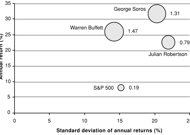
One of the great ironies in the annals of finance is that George Soros is probably the most misunderstood and controversial figure in the money man-agement scene. However, based on realized performance, he is probably the greatest investor the world has ever seen. This is ironic because George Soros’ sterling conversion trade in 1992 is considered as symptomatic of pure specu-lation. Soros compounded at an annual rate of 31.6 percent (after fees) in the 33 years from 1969 to 2001. This compares with around 26.0 percent in the case of Warren Buffett in the 44 years ending 2001 and with around 22.4 per-cent for Julian Robertson in the 22 years ending 2001. Note that compound-ing $1 at 31.6 percent, 26.0 percent, 22.4 percent and 7.9 percent (S&P 500) over a 25-year period results in terminal values of $958, $323, $157, and $6.7 respectively. This, albeit anecdotal, can be considered a big difference.

Who is the greatest money manager of all time? Most people would prob-ably agree that it is either George Soros or Warren Buffett. Figure 1.1 would suggest the former, Figure 1.2 the latter. Figure 1.2 shows annualized returns in relation to the standard deviations of these annual returns, that is, so-called risk-adjusted returns (implying that the standard deviation of returns is a sound proxy for risk). The sizes of the bubbles (and the numbers next to the

FIGURE 1.1 Performance of Greatest Long-Term Money Managers

Source:Hagstrom (1994), Peltz (2001), Datastream, TASS, Managed Account Reports. $1

$10 $100 $1,000 $10,000 $100,000 $1,000,000 $10,000,000 $100,000,000

1957 1962 1967 1972 1977 1982 1987 1992 1997 2002 Warren Buffett George Soros Julian Robertson S&P 500

$2.6m $19.7m

$2,871 $1.9m

FIGURE 1.2 Risk-Adjusted Returns of World’s Greatest Money Managers

Source:Hagstrom (1994), Peltz (2001), Datastream, TASS, Managed Account Reports.

1.47

1.31

0.79

0.19

0 5 10 15 20 25 30 35

0 5 10 15 20 25

Standard deviation of annual returns (%)

Ann

ual return (%)

Warren Buffett

George Soros

Julian Robertson

bubbles) measure the Sharpe ratios assuming a constant risk-free rate of 5 percent. Note that the risk-adjusted returns were calculated over different time periods.

Figure 1.1 and Figure 1.2 also reveal another interesting aspect of busi-ness life. According to Hagstrom (1994) Warren Buffett started with $100 in 1957. Figure 1.1 implies that his initial investment of $100 would have grown to only $2.6 million by the end of 2001. However, Warren Buffett is a multi-billionaire and one of the wealthiest individuals on the planet.* The differ-ence between $2.6 million and his X-billion wealth is attributed to entrepreneurism and not investment skill (albeit there is strong correlation be-tween the two). This should serve as a reminder to day traders and other fi-nancial comedians: Unambiguous greatness and sustainable value creation are achieved through successfully setting up and running businesses and not through having a go at the stock market.

The 1970s

Richard Elden (2001), founder and chairman of Chicago-based fund of (hedge) funds operator Grosvenor Partners, estimates that by 1971 there were no more than 30 hedge funds in existence, the largest having $50 million un-der management. The aggregate capital of all hedge funds combined was probably less than $300 million. The first fund of hedge funds, Leveraged Capital Holdings, was created by Georges Karlweis in 1969 in Geneva.19_This

was followed by the first fund of funds in the United States, Grosvenor Part-ners in 1971.

In the years following the 1974 market bottom, hedge funds returned to operating in relative obscurity, as they had prior to 1966. The investment community largely forgot about them. Hedge funds of the 1970s were differ-ent from the institutions of today. They were small and lean. Typically, each fund consisted of two or three general partners, a secretary, and no analysts or back-office staff.20_{The main characteristic was that every hedge fund}

spe-cialized in one strategy. (This, too, is different from today.) Most managers focused on the Alfred Jones model, long/short equity. Because hedge funds represented such a small part of the asset management industry they went

noticed. This resulted in relatively little competition for investment opportu-nities and exploitable market inefficiencies. In the early 1970s there were probably more than 100 hedge funds. However, conditions eliminated most.

The 1980s

Only a modest number of hedge funds were established during the 1980s. Most of these funds had raised assets to manage on a word-of-mouth basis from wealthy individuals. Julian Robertson’s Jaguar fund, George Soros’ Quantum Fund, Jack Nash from Odyssey, and Michael Steinhardt Partners were compounding at 40 percent levels. Not only were they outperforming in bull markets, but they outperformed in bear markets as well. In 1990, for ex-ample, Quantum was up 30 percent and Jaguar was up 20 percent, while the S&P 500 was down 3 percent and the Morgan Stanley Capital International (MSCI) World index was down 16 percent. The press began to write articles and profiles drawing attention to these remarkable funds and their extraordi-nary managers.

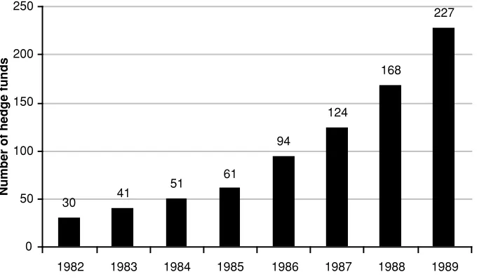
Figure 1.3 shows an estimate of number of hedge funds in existence through the 1980s. Duplicate share classes, funds of funds, managed futures, and currency speculators were not included in the graph.

During the 1980s, most of the hedge fund managers in the United States were not registered with the SEC. Because of this, they were prohibited from

FIGURE 1.3 Number of Hedge Funds in the 1980s

Source:Quellos Group.

30 41

51 61

94

124

168

227

0 50 100 150 200 250

1982 1983 1984 1985 1986 1987 1988 1989

Number of hedg

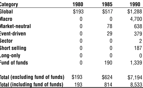
advertising, and instead relied on word-of-mouth references to grow their as-sets. (See Table 1.1.) The majority of funds were organized as limited partner-ships, allowing only 99 investors. The hedge fund managers, therefore, required high minimum investments. European investors were quick to see the advantages of this new breed of managers, which fueled the development of the more tax-efficient offshore funds.

Caldwell (1995) puts the date where hedge funds reentered the invest-ment community at May 1986, when Institutional Investorran a story about Julian Robertson.21 _{The article, by Julie Rohrer, reported that Robertson’s}

Tiger Fund had been compounding at 43 percent during its first six years, net of expenses and incentive fees. This compared to 18.7 percent for the S&P 500 during the same period. The article established Robertson as an investor, not a trader, and said that he always hedged his portfolio with short sales. One of the successful trades the article mentioned was a bet on a falling U.S. dollar against other major currencies in 1985. Robertson had bought an op-tion, limiting downside risk by putting only a fraction of the fund’s capital at risk. Rohrer showed the difference between a well-managed hedge fund and traditional equity management.

Another fund worth mentioning was Princeton/Newport Trading Part-ners. Princeton/Newport was a little-known but very successful (convertible) arbitrage fund with offices in Princeton, New Jersey, and Newport Beach, California. Some practitioners credit the firm with having the first proper op-tion pricing model and making money by arbitraging securities; this included optionality that other market participants were not able to price properly. For

Table 1.1 Hedge Fund Assets under Management in the 1980s ($ millions)

Category 1980 1985 1990 Global $193 $517 $1,288

Macro 0 0 4,700

Market-neutral 0 78 638

Event-driven 0 29 379

Sector 0 0 2

Short selling 0 0 187

Long-only 0 0 0

Fund of funds 0 190 1,339

Total (excluding fund of funds) $193 $624 $7,194

Total (including fund of funds) 193 814 8,533

two decades up to 1988, Princeton/Newport had achieved a remarkable track record with returns in the high teens and extremely few negative months. Un-fortunately, Princeton/Newport was hit by overzealous government action that led to an abrupt cessation of operations in 1988.*

The 1990s

During the 1990s, the flight of money managers from large institutions accel-erated, with a resulting surge in the number of hedge funds. Their operations were funded primarily by the new wealth that had been created by the un-precedented bull run in the equity markets. The managers’ objectives were not purely financial. Many established their own businesses for lifestyle and control reasons. Almost all hedge fund managers invested a substantial por-tion of their own net worth in the fund alongside their investors.

One of the characteristics of the 1990s was that the hedge fund industry became extremely heterogeneous. In 1990, two-thirds of hedge fund man-agers were macro manman-agers, that is, absolute return manman-agers with a rather loose mandate. Throughout the decade, more strategies became available for investors to invest in. Some of the strategies were new; most of them were not. By the end of 2001, more than 50 percent of the assets under manage-ment were somehow related to a variant of the Jones model, long/short eq-uity. However, even the subgroup of long/short equity became heterogeneous. Figure 1.4 compares some alternative investment strategies with the tradi-tional long-only strategy with respect to the variation in net market exposure. The horizontal lines show rough approximations of the ranges in which the different managers are expected to operate. It will become clear in later chap-ters that the superiority of the long/short approach is derived from widening the set of opportunities (and the magnitude of opportunities) from which the manager can extract value. The graph highlights a further aspect of hedge fund investing: Not all equity absolute return managers have the same invest-ment approach. This diversity results in low correlation among different man-agers, despite the managers trading the same asset class. Low correlation among portfolio constituents then allows construction of low-risk portfolios.

The 1990s saw another interesting phenomenon. A number of the es-tablished money managers stopped accepting new money to manage. Some even returned money to their investors. Limiting assets in many investment styles is one of the most basic tenets of hedge fund investing if the perfor-mance expectations are going to continue to be met. This reflects the fact that managers make much more money from performance fees and invest-ment income than they do from manageinvest-ment fees. Due to increasing in-vestor demand in the 1990s, many funds established higher minimum investment levels ($50 million in some cases) and set long lock-up periods (three to five years).

Both Julian Robertson’s Tiger Management and George Soros’ Soros Fund Management reached $22 billion in assets in 1998, setting a record for funds under management.22_{Both organizations subsequently shrunk in size,}

and Tiger ultimately was liquidated. Today, there are dozens of organizations managing more than $1 billion. Based on data from Hedge Fund Research, Inc. (HFRI) the hedge fund industry grew in terms of unleveraged assets un-der management of $38.9 billion in 1990 to $456.4 billion in 1999 and $536.9 billion at the end of 2001.

FIGURE 1.4 Different Strategies in Equities

Source:Quellos Group.

–150 –100 –50 0 50 100 150 200 250

Short-biased Market-neutral

Low beta Long-biased Opportunistic long/short

Traditional long-only

Conclusion

Some investors in the hedge fund industry argue that the pursuit of absolute returns is much older than the pursuit of relative returns (i.e., beating a benchmark). This view can be justified if we allow for a loose interpretation of historical deals. One could conclude that the way hedge funds manage as-sets is going back to the roots of investing. What Charles Ellis (1998) calls trying to win the loser’s game, therefore, could be viewed as only a short blip in the evolution of investment management. Put differently, both the first and third paradigm of investment management were about absolute returns.

Irrespective of the history of hedge funds or whether hedge funds are leading or lagging the establishment, the pursuit of absolute returns is probably as old as civilization and trade itself. However, so is lemming-like trend following.

INVESTMENT PHILOSOPHY OF ABSOLUTE

RETURN MANAGERS

Introduction

An absolute return manager is essentially an asset manager without a bench-mark or with a benchbench-mark that is the return on the risk-free asset. Bench-marking can be viewed as a method of restricting investment managers so as to limit the potential for surprises, either positive or negative. By defining a market benchmark and a tracking error band, the plan sponsor gives the manager a risk budget in which the manager is expected to operate. Recent le-gal action in the United Kingdom by a pension plan sponsor probably will mean that the relative return industry will be even more “benchmark-aware” than it already was.*

Separating skill from luck is one of the major goals of analyzing the per-formance of a particular manager, regardless of whether he is running long-only or absolute return money. In any sample of managers, a small percentage is bound to have exceptional performance (both positive and neg-ative). Managers with exceptional positive performance will attribute the ex-cess return to skill. Those who perform exceptionally poorly are unlikely to blame lack of skill but rather bad luck as the cause of their performance. Gri-nold and Kahn (2000a) categorize managers according to luck and skill. The

lucky and skilled are “blessed.” The lucky and unskilled are “insufferable.” The unlucky but skilled are “forlorn,” whereas the unlucky and unskilled are “doomed.”

Grinold and Kahn argue that “nearly half of all roulette players achieve positive returns on each spin of the wheel.” This means that the wheel most often stops on red or black (as opposed to 0 or 00). Even the existence of very large returns (such as when the ball stops on a single number bet like 7) does not prove skill. However, the expected return of the roulette gambler is nega-tive. Over the long term, they all lose. The casino, however, has positive ex-pected returns and wins (as long as it has enough cash or credit lines to live through a bad evening).*

The practical issue arising from performance analysis is that it requires a certain amount of data points before any conclusions can be drawn with a reasonable degree of confidence. For example, to analyze yearly returns, 16 years of observations are needed to judge whether a manager is top quartile (has an information ratio of 0.5) with 95 percent confidence. As the normal life span of an asset manager is less than 16 years, a 16-year monitoring pe-riod seems rather impractical. Assessing qualitative aspects (investment phi-losophy, trading savvy, risk management experience, infrastructure, incentive structure, etc.)—that is, bottom-up fundamental research and due diligence— is the only way around this issue.

A Car without Brakes

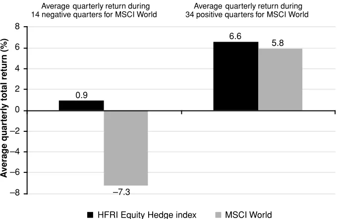
The most comparable strategy to long-only equity is long/short equity. The HFRI Equity Hedge Index (equity long/short managers) outperformed most equity market indexes on an absolute as well as risk-adjusted basis by a wide margin. However, most long/short managers should underperform long-only managers in momentum-driven bull markets where all stocks increase rapidly.†_{The long/short manager should underperform because the short}

po-sitions are a drag on performance (for example, in liquidity-driven momen-tum markets as in the late 1990s). However, when markets have only slightly positive or negative returns, long/short managers have outperformed the

*Running a casino, an insurance company, or the national lottery is a business called statistical arbitrage. The operators win as long as they can survive statistical outliers, that is, large but few occasional outflows or losses. Statistical arbitrage is one strategy executed by absolute return managers. The irony is that the public perceives absolute return managers to be like gamblers, whereas they are actually more like someone run-ning a casino. Their expected return is positive.

†_{Note that this is a generalization and that generalizations are actually inappropriate}

long-only managers, at least in the past. In other words, long/short hedge funds underperform in strong bull markets and outperform in bear markets. This means that if the returns of the benchmark index are fairly normally dis-tributed, the return profile of absolute return managers is nonlinear, that is, asymmetrical to the market. Figure 1.5 shows the symmetrical returns of an equity index and compares it with the asymmetrical return profile of a hedge fund index. The figure shows the average quarterly returns of the HFRI Eq-uity Hedge Index when the MSCI World was positive and negative respec-tively. The average of the 34 positive quarterly returns between 1990 and 2001 was 5.8 percent. The corresponding return for the HFRI Equity Hedge Index was 6.6 percent. The averages of the 14 negative quarters were –7.3 percent and 0.9 percent respectively.

The main reason why traditional funds do more poorly in downside mar-kets is that they usually need to have a certain weight in equities according to their mandate, and therefore are often compared to a car without brakes. The freedom of operation is limited with traditional asset managers and more flexible with absolute return managers. Another reason why hedge fund man-agers may do better in down markets is that they often have a large portion of their personal wealth at risk in their funds. Arguably, their interests are more aligned with those of their investors. This alignment, together with the lack of

FIGURE 1.5 Asymmetrical versus Symmetrical Return Profile, 1990–2001

Source: Hedge Fund Research, Datastream, UBS Warburg (2000).

0.9

6.6

5.8

–8 –6 –4 –2 0 2 4 6 8

A

vera

g

e

quar

terl

y total return (%)

HFRI Equity Hedge index MSCI World Average quarterly return during

14 negative quarters for MSCI World

Average quarterly return during 34 positive quarters for MSCI World

a relative measure for risk, increases the incentive to preserve wealth and avoid losses.

Avoiding Negative Compounding

Downside protection is closely related to avoiding negative compounding. A simple example may help illustrate the importance of wealth preservation: If one loses 50 percent, as various markets and stocks did during 2000–2001, one needs a 100 percent return just to get back to breakeven. That is, the pos-itive return must be double the negative return. We argue that downside pro-tection from the investors’ point of view and avoidance of negative returns from the managers’ point of view are different sides of the same coin.

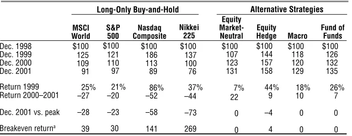
Table 1.2 is an attempt to explain the investment philosophy of ab-solute return managers. Both abab-solute and relative return managers would argue that they were not hired by investors to lose money. The fundamental difference between the two investment philosophies lies in the aversion to absolute financial losses and the definition of risk. Absolute return man-agers define risk as total risk whereas relative return managers define risk as active risk.

Orthodox financial theory suggests that investors should focus on the long term. It also suggests that investors will generate satisfactory returns if they have a long enough time horizon when they buy equities. This may or may not be true. The problem faced by absolute return managers is that they might not live long enough to experience the long term. Absolute return man-agers do not care if the probability of equities underperforming bonds over a 25-year period is low. Moreover, absolute return managers are interested in

Table 1.2 Different Approaches to Creating Value

MSCI World

S&P 500

Nasdaq

Composite Macro

Dec. 1998 $100 $100 $100 $100 $100 $100 $100 $100

Dec. 1999 125 121 186 137 107 144 118 126

Dec. 2000 109 110 113 100 123 157 120 132

Dec. 2001 91 97 89 76 131 158 129 135

25% 21% 86% 37% 7% 44% 18% 26%

–27 –20 –52 –44 22 9 10 7

–28 –23 –58 –73 0 –4 0 0

39 30 141 269 0 4 0 0

Alternative Strategies Long-Only Buy-and-Hold

Breakeven returna

Dec. 2001 vs. peak Return 2000–2001 Return 1999

Nikkei 225

Equity Market-Neutral

Equity Hedge

Fund of Funds

a_{Return required to break even from previous peak.}

how they get there; that is, they are interested in end-of-periodwealth as well as during-the-periodvariance.

Table 1.2 summarizes what we mean by “avoiding negative compound-ing.” It shows four long-only buy-and-hold portfolios as well as four alterna-tive absolute return strategies. The absolute return manager could argue that the first four columns have nothing to do with asset management or risk man-agement. Absolute return managers want to make profits not only when the wind is at their backs but also when it changes and becomes a headwind. Ab-solute return managers will therefore use risk management and hedging tech-niques—this is where the asymmetrical return profile discussed earlier comes from. From the point of view of absolute return managers, relative return managers do not use risk management,* and do not manage assets as they follow benchmarks. They are trend followers by definition.

In other words, the relative return manager is long; hence the term long-only. The relative return manager, again from the point of view of the absolute return manager, has no incentive, no provisions to avoid losses.†

This does not make sense to many absolute return managers and is the rea-son why some absolute return managers believe relative return managers face obsolescence.

Table 1.2 shows that an investment in the four equity indexes in December 1998 would have ended in losses by December 2001, despite the phenomenal performance of equities in 1999.‡ _{The second row from the bottom measures}

the percentage from the peak in local currencies. The high losses in the Nikkei 225 make it clear why some Japanese investors are not as averse to hedge fund exposure as are, for example, U.K. pension fund trustees. (Demand for hedge fund products is larger from Japanese institutional investors than it is from U.K. institutional investors.) It also illustrates one of the incentives of absolute return managers. Absolute return managers would try to keep this figure at zero, because first they have their own money in the fund and do not want to lose it, and second, most hedge fund managers have a high-water mark. This

*Note that, for example, Lo (2001) expresses a diametrically opposing view, arguing that “risk management is not central to the success of hedge funds” whereas “risk management and transparency are essential” for the traditional manager.

†_{This is not entirely correct: A relative return manager has an incentive to grow funds}

under management (i.e., avoid funds under management falling) because fee income is determined based on the absolute level of funds under management.

‡_{It is interesting to note that some fund of hedge funds managers regard themselves as}

means that they can charge an incentive fee only from new profits; that is, the fund has to make up for any losses before it can charge its performance fee. For example, a fund falling to 80 from 100 and then rising back to 100 will not charge a performance fee on the 25 percent profit from 80 to 100.

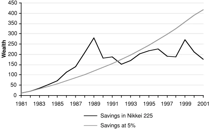
Figure 1.6 shows two hypothetical saving schemes of a Japanese em-ployee, assuming deposits are made at the end of each calendar year over a 20-year period and that deposits grew 2 percent per annum due to salary in-creases. The two series contrast a local stock market savings scheme (as mea-sured by the Nikkei 225) and a fixed-rate scheme of 5 percent. Figure 1.6 should serve as a reminder that it is true that equity markets go up in the long term but: (1) Differences between markets are huge. Taking the S&P 500 as a proxy for equity investing over the past 10, 20, 50, or even 100 years is inap-propriate because the U.S. stock market is the mother of all stock markets, that is, the winner of a large group of survivors. (2) An investor might not live long enough to experience the long term.

Nearly all analysis in the asset management industry is based on time-weightedrates of return. However, the most relevant metric from an investor’s perspective is dollar-weighted rates of return or their internal rate of return (IRR). For example, Manager A earns 20 percent, 20 percent and –10 percent in years one to three, while Manager B earns –10 percent, 20 percent, and 20 percent. In both cases, the time-weighted return is the same (9 percent average

FIGURE 1.6 Low Volatility Savings Plan Compared with Equity Investment

Source:Datastream.

0 50 100 150 200 250 300 350 400 450

1981 1983 1985 1987 1989 1991 1993 1995 1997 1999 2001

W

ealth

Savings in Nikkei 225

annual compound growth). However, the dollar-weighted rate of return be-tween the two managers will likely be vastly different for nearly all investors. The only exception is investors that neither invest nor withdraw assets. These investors would have earned the same IRR by investing with either manager. An investor who was a saver, contributing $100 per year, would earn $120, $264, and $328 with Manager A by the end of years one to three, respectively, but $90, $228, and $394 with Manager B. The increase in wealth produced by each fund ($328 versus $394) is dramatically different even though the time-weighted return is the same. This effect is more pronounced the greater the de-gree of variation in returns. Earning 9 percent per year results in $357 at the end of period three, that is, is in between the two other outcomes. Accumula-tion of wealth is much more reliable (less risky) the lower the total risk.

Assume that the dark line in Figure 1.6 is the retirement plan of a 45-year-old employee who started working 20 years ago and has been investing money in the stock market every year, starting with $10 in year one. The employee’s wealth would have been $241 at the end of 2001. Invested at 5 percent, this would have ended in wealth of $416 (assuming contribution increases at a rate of 2 percent in both cases). In other words, the stock market has not been that great for a Japanese saver over the past 20 years, despite the fact that the 1980s was one of the greatest bull markets ever in the country’s financial history (as were the 1990s in the United States and Europe).* If the hypothetical Japanese equity saver continues to get a salary increase of 2 percent per year and invests it in the Nikkei 225, the annual growth rate of the Nikkei 225 over the next 20 years has to be around 9.6 percent to equal the fixed-rate investment over the full 40-year period. If this growth rate materializes, the Japanese investor would be as well positioned at retirement age 65 as if he or she had invested at 5 per-cent. The Japanese equity market might perform at a rate of 9.6 percent per year over the next 20 years; however, and this is the whole point, it might not.†

The Nikkei 225 is an extreme example that was chosen on purpose. The choice is based on the fact that the high volatility in equity markets can have a large impact on end-of-period wealth as well as variance during the invest-ment period. An investinvest-ment strategy that does not manage both end-of-period

*For this not to happen to savers in the United States and Europe there is an urgent need of incremental buyers, that is, buyers who consider valuations in the high thirties or low forties—based on aggregate market earnings per share (EPS)—as cheap. Conti-nental European pension funds have been announcing throughout the late 1990s that they will increase their allocations to equities. Most investors and financial profession-als hope that they do not change their minds. For a market to go up, there is a need for (incremental) buyers. No buyers—no asset price inflation.

†_{At a rate of 9.6 percent per year, the Nikkei 225 would break through its all-time high}

wealth as well as during-the-period variance is not an active but rather a pas-sive investment strategy.

Return Illusion

To the casual observer, the return of 86 percent on the Nasdaq index in Table 1.2 may look high even if it is followed by a retreat of only52 percent. How-ever, if $100 had been passively invested in the Nasdaq Composite index at the beginning of 1999 and transaction costs were zero, the portfolio would have declined to $89 by the end of December 2001 (an $86 gain in 1999 followed by a $97 loss in 2000–2001). This compares with $131 for a portfolio of eq-uity market-neutral absolute return managers, $135 for the average fund of hedge funds, or $129 for a diversified exposure to global macro managers.* High returns as observed on the Nasdaq are good for headlines and selling fi-nancial magazines. However, these returns are an illusion in a long-term con-text. A volatile market-based strategy with returns such as 89 percent per year is an indication that the return figure might reverse in a linear fashion.

The figures in Table 1.2 are only moderately conclusive because the analysis has starting- and end-point bias. However, a point worth making is that investing in absolute return funds or adding alternative asset classes and strategies to traditional asset classes and strategies is a conservative undertak-ing. Diversifying into assets with low correlation to one’s existing assets or combining assets with low correlation reduces total risk. Diversification and hedging unwanted risks are laudable concepts—despite the popular belief that, apparently, (still) suggests otherwise: In the United States, 401(k) plans allow a 100 percent allocation to one stock. In the United Kingdom, some pension funds recently had a larger allocation to one domestic stock than to the whole U.S. stock market due to benchmark considerations. It is unlikely that these examples of suboptimal allocation of risk will persist forever.

Perception of Risk

Misunderstanding about absolute return managers is derived from the ob-servation that relative and absolute return managers do not speak the same

language. Terminologies and perceptions can be as different as the strate-gies. One perception has to do with risk. When a relative return manager speaks of risk he or she normally means active risk. When an absolute re-turn manager speaks of risk he or she usually means total risk, that is, the probability of losing everything and being forced to work for a large organi-zation again.

Traditional long-only managers whose benchmark is, for example, the S&P 500 see a “riskless” position as holding all 500 stocks in exact proportion as the index. Shifting 10 percent out of high-beta stocks into cash is perceived as an in-crease in risk. Absolute return managers would view such a shift as decreasing risk. In other words, absolute return managers have a different perspective.

This does not mean that a relative return manager perceives true financial risk as active risk. Losing money is obviously worse than making money. However, it is active risk that is linked to their remuneration and future career prospects. Their incentive and mandate is to manage active risk, not total risk. The investment consulting boom beginning in the late 1960s and the pa-per on asset allocation by Gary Brinson et al. (1986) were probably the key moments in the bifurcation of the second paradigm of asset allocation, that is, the migration from an absolute return to a relative return perspective. Institu-tional investors, academics, and consultants were the drivers pushing money managers to assimilate the relative perspective toward risk and return— whether long-only managers liked it or not. The third paradigm in asset man-agement mentioned in the Preface is steering away from the odd incentives derived from a relative return approach.

Risk Illusion from Time Diversification

An often-debated phenomenon in equity markets is the benefit of time diversifi-cation. Some argue that equities are safe in the long term.* The argument goes as follows: Equities have a 60 percent probability of outperforming government

bonds over a one-year period and a 95 percent outperformance probability over 25 years. In addition, long-term volatility is normally lower than short-term volatility. The apparent conclusion, therefore, is that investing in equities is foolproof as long as one has a long time horizon. The debate surrounding whether time reduces risk is often referred to as the time diversification contro-versy. Another school of thought argues that time diversification is an illusion and a longer time horizon does not reduce risk.

The illusion (or misconception) of time reducing risk arises from a misun-derstanding of risk. It is true that the annual average rate of return has a smaller standard deviation for a longer time horizon. However, it is also true that the uncertainty compounds over a greater number of years. Unfortu-nately, this latter effect dominates in the sense that the total return becomes more uncertain the longer the investment horizon. Had a long-term investor with a 100-year investment horizon decided to put money into the U.S. stock market in 1900, the investment would have compounded at a reasonable rate. However, other choices were other large markets such as Argentina, Imperial Russia, or Japan. The 100-year return of these markets was materially differ-ent than the U.S. experience.

An eye-opener is the difference between the probability of suffering a loss at the end ofthe investment period and the probability of suffering a loss dur-ing the investment period. The former is very small and the latter large by comparison. The practical significance is that large absolute losses are very uncomfortable for most investors, private as well as institutional. The differ-ence between 15 percent and 18 percent rates of return seems relatively small. The impact on ending wealth is considerably larger ($3,292 versus $6,267 compounded over 25 years for a $100 initial investment). Thus the variation or risk in end-of-period wealth does not decrease with time. Further, this analysis specifies no utility function for the investor. If an investor had uncer-tainty as to when he or she would withdraw money, the variability in ending wealth would further diminish the value of the risky investment over the safer investment. End of the period and during the periodlose significance if the end of the investment period is not known with 100 percent certainty.

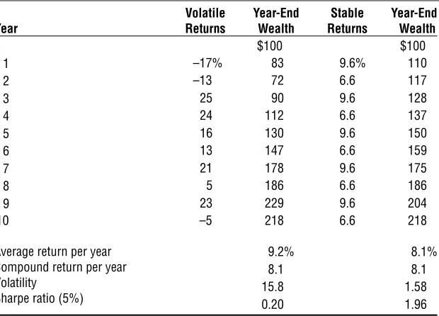
The financial industry has not yet paid a lot of attention to risk-adjusted returns. Pure returns or, in some cases, active returns are the main focus point when performance is presented to investors and/or prospects. With Table 1.3 we try to make the point that two portfolios with the same return are not nec-essarily the same.

the 10-year period covered a large part of the 1990s, which is generally considered to be one of the greatest decades for equity investors in the his-tory of financial markets.

The view of an absolute return manager is that many investors underesti-mate the impact of negative years on overall wealth creation. The first strat-egy in Table 1.3 looks superior because the average of the simple returns is 9.2 percent whereas it is only 8.1 percent for the second strategy. However, once the compound annual return of 8.1 percent is put into context with the variance of the returns, the investment with the stable returns does not appear to be inferior. As a matter of fact, if end-of-period wealth as well as during-the-period variance matter, the investment with the more stable returns is su-perior.*

Many absolute return managers probably subscribe to Benjamin Gra-ham’s rule of investing:

Table 1.3 Volatile versus Stable Returns

$100 $100

1 –17% 83 9.6% 110

2 –13 72 6.6 117

3 25 90 9.6 128

4 24 112 6.6 137

5 16 130 9.6 150

6 13 147 6.6 159

7 21 178 9.6 175

8 5 186 6.6 186

9 23 229 9.6 204

10 –5 218 6.6 218

9.2% 8.1%

8.1 8.1

15.8 1.58

0.20 1.96

Volatile Year-End Stable Year-End Year Returns Wealth Returns Wealth

Average return per year Compound return per year Volatility

Sharpe ratio (5%)

The first rule of investment is don’t lose. And the second rule of invest-ment is don’t forget the first rule. And that’s all the rules there are.

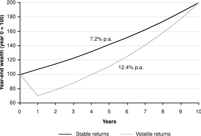
Today this is considered Wall Street wit and regularly used for ment purposes. However, the notion has probably more than just entertain-ment value. It is the reason why absolute return managers are more than just relative return managers with cash as their benchmark. It is also the reason why many investors regard investing to be at least as much alchemy (Soros, 1987) or art (Yale Endowment, 2001) as it is pure science. Figure 1.7 shows that portfolio volatility matters.

Figure 1.7 shows two 10-year investments that double over a 10-year pe-riod. The dark line is a $100 investment growing at 7.2 percent over the 10-year period. The lighter line experiences a loss of 30 percent in the first 10-year. The growth rate to match the 7.2 percent growth rate in the remaining nine years is 12.4 percent. If the second investment grew from 70 after the first year at a rate of 7.2 percent, the end-of-period wealth would accumulate to only $131. The annualized return would result in a compounded annual growth rate of only 2.7 percent. To an absolute return manager, an invest-ment vehicle where there is no provision to manage volatility is, to use the po-litically correct term, suboptimal. Note that in many continental European

FIGURE 1.7 Different Ways of Doubling an Initial Investment of $100

60 80 100 120 140 160 180 200

0 1 2 3 4 5 6 7 8 9 10

Years

Y

ear

-end wealth (y

ear 0 = 100)

Stable returns Volatile returns 7.2% p.a.

countries the equity culture began in the late 1990s. It is not unreasonable to assume that for some investors the 2000–2002 bear market was the first expe-rience with equities as an asset class.

Managing Volatility

Putting it crudely: Absolute return managers have an incentive to manage volatility, whereas only managers do not. The portfolios of most long-only managers closely track the benchmark. When the benchmark has a volatility of around 10 percent (as some developed equity markets had around 1995), then the portfolio of the long-only manager will have a volatil-ity of 10 percent. When the volatilvolatil-ity of the benchmark increases to 25 per-cent (as in most developed markets in the period 1997 to 2000), then the portfolio of the long-only manager will have a volatility of around 25 percent. This makes sense because it is in line with the mandate (i.e., mimicking the benchmark market index). Whether this makes sense on a more general level is, for the time being, in the eye of the beholder.

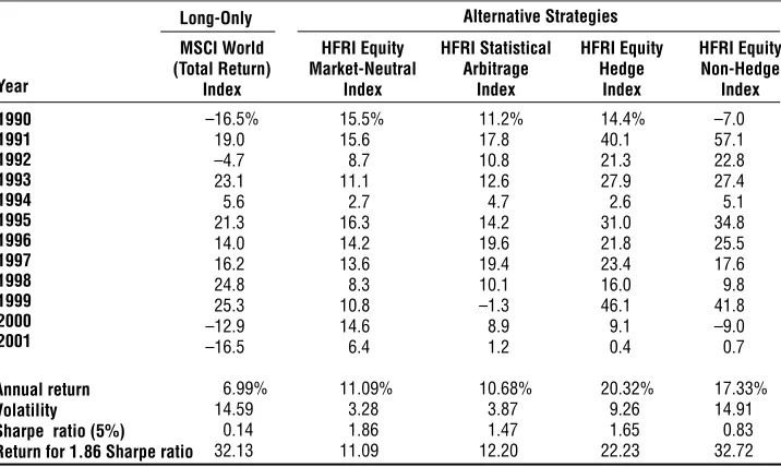
Table 1.4 shows five different ways of managing equity risk. The first is the traditional long-only way where there is no incentive to hedge market risk. The MSCI World index was used as a proxy for a long-only portfolio.

Table 1.4 Long-Only Compared with Market-Neutral and Long/Short Equity

Long-Only

MSCI World HFRI Equity HFRI Statistical HFRI Equity HFRI Equity (Total Return) Market-Neutral Arbitrage Hedge Non-Hedge

Index Index Index Index Index

–16.5% 15.5% 11.2% 14.4% –7.0

19.0 15.6 17.8 40.1 57.1

–4.7 8.7 10.8 21.3 22.8

23.1 11.1 12.6 27.9 27.4

5.6 2.7 4.7 2.6 5.1

21.3 16.3 14.2 31.0 34.8

14.0 14.2 19.6 21.8 25.5

16.2 13.6 19.4 23.4 17.6

24.8 8.3 10.1 16.0 9.8

25.3 10.8 –1.3 46.1 41.8

–12.9 14.6 8.9 9.1 –9.0

–16.5 6.4 1.2 0.4 0.7

6.99% 11.09% 10.68% 20.32% 17.33%

14.59 3.28 3.87 9.26 14.91

0.14 1.86 1.47 1.65 0.83

32.13 11.09 12.20 22.23 32.72

Alternative Strategies

Annual return Volatility Sharpe ratio (5%) Return for 1.86 Sharpe ratio Year

1990 1991 1992 1993 1994 1995 1996 1997 1998 1999 2000 2001

The four other equity strategies involve managing downside market risk to different degrees. The HFRI Equity Market-Neutral and HFRI Statistical Ar-bitrage indexes are both relative value strategies where market risk is fully hedged at all times. The other two strategies are long/short strategies. In eq-uity hedge managers have a small long bias, and in eqeq-uity nonhedge there is a large long bias. Of these five investments, the market-neutral one has the highest risk-adjusted returns whereas the MSCI World index has the lowest. Assume an investor has a risk budget for equitylike risk, which one of the five investments is superior over the other four?

As shown in Figure 1.8, the five (capital market) lines originate at the risk-free rate, which is most often assumed to have zero risk.* Each line is drawn through the risk/return point in the graph. The steepest line is consid-ered the best. It is not important where the dot is. The reason why the posi-tion of the dot is irrelevant is because of the use of leverage. If an investor has a risk budget (risk appetite) of 9.26 percent as the second best investment in Figure 1.8, he could borrow money and invest in the best investment.

Assum-*An investment at the risk-free rate is considered risk free. However, volatility is not zero. The ambiguity derives from the fact that in financial theory volatility (annualized standard deviation of returns) is used as a proxy for risk.

FIGURE 1.8 Risk/Return Trade-off of Five Equity Investment Styles

Source: Hedge Fund Research, Datastream.

0 5 10 15 20 25

0 2 4 6 8 10 12 14 16

Volatility (%)

ing the investor borrows money at the risk-free rate, invests in the best invest-ment, and accepts a volatility of 9.2 percent, the resultant return would be around 22.2 percent, that is, approximately 190 basis points higher than the second best investment with the same volatility. If the investor is ready to ac-cept the volatility of the most volatile investment (which also happens to be the worst investment of the five), that is, a volatility of 14.59 percent, he or she can lever up and invest in the best investment. The return of using lever-age and investment in the best investment would result in an annual return of around 32.1 percent. This seems to represent a big difference from the 7.0 percent in the MSCI World.

Where does this analysis fail? There must be something wrong. First, hedge fund data is inflated for various reasons discussed in later chapters. In addition, volatilities are most likely too low; that is, Sharpe ratios too high. However, these measurement imperfections are unlikely to explain the 2,471 basis points between the best investment in Figure 1.8 and the worst. Second, there is a capacity issue. The worst investment in Figure 1.8 has a market capitalization in excess of $25 trillion whereas the best invest-ment is probably around $50 billion.* What would happen if the investors holding the $25 trillion were to rebalance their portfolio by moving funds from the worst investment to the best investment? The capital market lines would move. Putting it crudely: The suppliers of the $50 billion can deliver Sharpe ratios of 1.86 only if the holders of the $25 trillion do not mind having a Sharpe ratio of 0.14. If the holders of $25 trillion decide tomor-row that a Sharpe ratio of 1.86 is more appealing than a Sharpe ratio of 0.14, then the suppliers of a Sharpe ratio of 1.86 will get flooded with funds. In other words, once all investors start requesting higher Sharpe ra-tios, the capital market lines in Figure 1.8 will converge. The suppliers of a Sharpe ratio of 1.86 for $50 billion will, by definition, not be able to de-liver a Sharpe ratio of 1.86 for $25 trillion. The pioneers of absolute return strategies were enjoying an economic rent that cannot be supported if $25 trillion was managed in this format. Superior risk-adjusted returns—that is, superior performance—attracts capital. Assuming alpha is finite, the al-pha will be spread over more investors going forward.†_{This means that}

un-locking the alpha in the hedge fund industry is becoming more difficult over time.

*Assuming around 10 percent of the hedge funds universe is market-neutral (or is de-livering a Sharpe ratio of 1.86 on a consistent and sustainable basis).

†_{Unless the regulator intervenes, that is. If regulators only allow certain investors to}

Conclusion

The investment philosophy of absolute return managers differs from that of relative return managers. Absolute return managers care not only about the long-term compounded returns on their investments but also how their wealth changes during the investment period. In other words, an absolute return manager tries to increase wealth by balancing opportunities with risk, and run portfolios that are diversified and/or hedged against strong fluctuations. To the absolute return manager these objectives are consid-ered conservative.

DEFINING THE HEDGE FUND INDUSTRY

Definition

There are nearly as many definitions of hedge funds as there are hedge funds. We define a hedge fund as follows: A hedge fund constitutes an investment program whereby the managers or partners seek absolute returns by exploit-ing investment opportunities while protectexploit-ing principal from potential finan-cial loss. With this definition we capture the balancing act of the absolute return manager. On one hand, the absolute return manager tries to make money by exploiting investment opportunities. However, the profit opportu-nity is always put into context with the potential loss of principal. (Note that this definition does not apply for the relative return manager where the goal is to beat a benchmark.) Crerend (1995) defines hedge funds as follows:

Hedge funds are private partnerships wherein the manager or general partner has a significant personal stake in the fund and is free to operate in a variety of markets and to utilize investments and strategies with vari-able long/short exposures and degrees of leverage.

Unfortunately, not all hedge fund managers have “a significant personal stake” in the fund. Nonetheless, beyond the basic characteristics embodied in this definition, hedge funds commonly share a variety of other structural traits. They are typically organized as limited partnerships or limited liability companies. They are often domiciled offshore, for tax and regulatory reasons. And, unlike traditional funds, they are not as much burdened by regulation. Less regulation means less protection for the investor and more flexibility for the hedge fund manager. Less protection means higher risk for the investor, for which the investor seeks compensation.