R E S E A R C H
Open Access
Missing in space: an evaluation of imputation
methods for missing data in spatial analysis of
risk factors for type II diabetes
Jannah Baker
1,2*, Nicole White
1,2and Kerrie Mengersen
1,2Abstract
Background:Spatial analysis is increasingly important for identifying modifiable geographic risk factors for disease. However, spatial health data from surveys are often incomplete, ranging from missing data for only a few variables, to missing data for many variables. For spatial analyses of health outcomes, selection of an appropriate imputation method is critical in order to produce the most accurate inferences.
Methods:We present a cross-validation approach to select between three imputation methods for health survey data with correlated lifestyle covariates, using as a case study, type II diabetes mellitus (DM II) risk across 71 Queensland Local Government Areas (LGAs). We compare the accuracy of mean imputation to imputation using multivariate normal and conditional autoregressive prior distributions.
Results:Choice of imputation method depends upon the application and is not necessarily the most complex method. Mean imputation was selected as the most accurate method in this application.
Conclusions:Selecting an appropriate imputation method for health survey data, after accounting for spatial correlation and correlation between covariates, allows more complete analysis of geographic risk factors for disease with more confidence in the results to inform public policy decision-making.
Keywords:Imputation, Missing, Spatial, Prevalence, Diabetes
Background
Spatial analysis is being used increasingly to identify geo-graphic risk factors associated with disease and areas at high excess risk of disease beyond what would be expected given the prevalence of these risk factors. Many geographic risk factors are modifiable and amenable to health promo-tion programmes, thus spatial analysis can provide useful information to inform resource allocation and public policy decisions. Maps of spatial models have been useful for highlighting differential risk across regions. They are par-ticularly useful for small area estimation, since the accuracy and precision of estimates based on small counts in a region can be improved by “borrowing strength” from estimates in neighbouring regions [1]. Bayesian models are particularly well suited to spatial modelling since the
information provided by neighbouring regions can be naturally represented as priors [2].
Routinely collected survey data can provide useful information about the distribution of covariates at a regional level, but frequently a problem with such data is the presence of missing covariate information. Often the data are spatially correlated and/or there are correlations between covariates. In these cases, imputation of missing data with plausible values allows inferences to be made about outcomes and covariates using statistical methods suited to complete data. Several methods of imputation are available and it is important to select the one best suited to a particular dataset.
In this paper, we address this challenge by considering a case study of geographic risk factors associated with type II diabetes (DM II).
The prevalence of DM II is increasing worldwide, with a report from Diabetes UK reporting a“state of crisis”in diabetes care [3]. Diabetes is reported to affect 11.3% of * Correspondence:[email protected]
1
Queensland University of Technology School of Mathematical Sciences, Brisbane, Australia
2
Cooperative Research Centres for Spatial Information, Melbourne, Australia
the US and 4.45% of the UK adult population, of which DM II accounts for 90-95% of cases [3,4]. Diabetes is reported to be the leading cause of renal failure, non-traumatic lower-limb amputation, and new cases of blindness, the major cause of heart disease and stroke, and the seventh leading cause of death in the US [4].
Despite the rising shortage of service provision for DM II, there is evidence that DM II is preventable in 60% cases with lifestyle change and/or medications [5]. Thus long-term consequences of DM II can be pre-vented through early detection and management of glycaemic control and cardiovascular risk factors [6]. Evidence shows that DM II is associated with both en-vironmental and individual factors [7]. Therefore, ana-lysis of geographic differences in DM II incidence may provide important information for more targeted inter-vention and management, and hence may be useful for informing resource allocation decisions.
Demographic and lifestyle factors associated with in-creased risk of developing DM II include male gender, increasing age, increasing BMI, increasing waist:hip ra-tio, indicators of low socio-economic status, sedentary lifestyle, physical inactivity, smoking history, and low levels of fruit and vegetable consumption [8-12]. In addition, spatial studies of DM II that aim to describe changes in DM II outcomes over a set of neighbouring regions have shown DM II to be associated with deprivation [12], socioeconomic status [9,11,13,14] and smoking prevalence [11] at a regional level. However, these studies have only been conducted in a very lim-ited number of countries to date. Moreover, there is a lack of spatial studies examining the association of DM II relative risk (RR) with the distribution of other can-didate lifestyle factors such as overweight/obesity, physical activity levels and fruit and vegetable con-sumption at a regional level.
Spatial studies examining DM II outcomes over regions have been developed in the US, England and Europe [7,9,11-18]. Spatial models estimated by Bayesian methods have successfully been used to model several diseases in-cluding DM II (Liese, Chaix, Congdon, Bayesian GLMMs), anaemia [19], dental caries [20], leprosy [21], multiple sclerosis [22], cancer incidence and mortality risk [23-25], malaria [26-28], and childhood leukaemia and lymphoma [29]. In our case study, we fit Bayesian spatial models to DM II prevalence data across Queensland regions, accounting for significant missing data.
This study has four objectives: a) to trial and select an appropriate imputation method to account for missing survey data from a number of relevant choices, b) to exam-ine geographic disparities in DM II RR in Queensland, b) to identify areas with high DM II RR in this region, and d) to identify environmental risk factors for DM II RR at a regional level.
Methods
For clarity, we first introduce the case study, then consider imputation methods, and finally evaluate these alternative methods in the context of the case study.
Case study
This case study examines disparities in the RR and relative excess risk (RER) of DM II across 71 Queensland LGAs, accounting for seven geographic lifestyle factors, after selection of the most appropriate imputation method out of three alternative methods. RR is defined as the ratio of the estimated risk in a particular LGA to the mean esti-mated risk across all LGAs; thus LGAs with a larger RR are estimated to be more at risk for DM II prevalence than LGAs with smaller RRs. RER is defined as the estimated excess risk for DM II prevalence in a particular LGA after taking into account the effect of lifestyle covariates in that region. Thus LGAs with a larger RER have unexplained higher risk for DM II prevalence than would be expected and may benefit more from programmes for early detec-tion and management of DM II.
Sources of data
Our analysis of the region-level determinants of DM II relative risk relied on three databases, briefly described below.
(1) The National Diabetes Services Scheme (NDSS) database for 2011 diabetic notification data [30]. The NDSS delivers diabetes-related products, information and support services to almost 1.1 million Australian with diabetes and monitors the prevalence of diabetes including DM II across regions in Australia. This database also contains 2011 data originally from the Australian Bureau of Statistics (ABS) for a) socioeconomic status (SES) measured by average income scored 1–10 (1 indicating lowest and 10 indicating highest income decile across Australia) and b) proportion over the age of 45 years for the general population in each LGA in Queensland, which were used as covariates in this case study. (2) The 2011 census information from the ABS for
estimated resident population (ERP) per LGA [31]. The ABS collects and publishes census data and monitors population counts across regions in Australia. (3) The Queensland self-reported health status
health benefit, adequate fruit intake (2+ serves/day), and adequate vegetable intake (5+ serves/day). The proportion overweight or obese in each LGA, defined as BMI≥25kg/m2, was estimated from self-reported height and weight.
The survey provides a total of 16,530 completed computer-assisted telephone interviews across Queensland, with a response rate of 56.7% in 2009 and 64.5% in 2010. The telephone numbers selected for this survey were reportedly sourced by random digit dialling (RDD) using a specific sample frame from the Association of Market and Social Research Organisations RDD sample database. Data are reported for LGAs that had a sample of 60 or more completed interviews (Brisbane LGA had the largest number of interviews at 2,561). Data are not reported from this survey for 28 LGAs with a sample size smaller than 60 due to potential inaccuracy of estimates.
The reported overall prevalence of DM II across all Queensland LGAs from NDSS data were combined with ERP data to compute estimated counts for each LGA. Three island LGAs (Mornington, Palm Island and Torres Strait Island) were excluded, leaving 71 Queensland LGAs included in this spatial analysis.
Ethical Statement
The QUT University Human Research Ethics Committee assessed this research as meeting the conditions for ex-emption from HREC review and approval in accordance with section 5.1.22 of the National Statement on Ethical Conduct in Human Research (2007). Exemption number: 1400000354 QV reference no.: 44305.
Spatial model
Multivariable models including all seven lifestyle covariates were fitted to the DM II prevalence data.
Bayesian generalised linear mixed models (GLMMs) using Markov chain Monte Carlo (MCMC) were used to model RR and prevalence across regions. Two general models were considered: a Binomial model and a Poisson model. The Binomial GLMMs took the form:
YieBin pð i;niÞ
logit pð Þ ¼i αþxiβþUiþSi ð1Þ
where for regioni,Yiis the observed number of DM II cases,pi is the estimated prevalence of DM II, andniis the estimated resident population. αis a fixed intercept,
βis a vector of coefficients, and xiis theith row of the design matrix X, containing covariate data for region i. The uncorrelated error for regioni is denotedUi, andSi is the correlated spatial error based on neighbourhood information; this is described in more detail below.
Separating the residual error into spatial (Si) and non-spatial (Ui) components provides an indication of how much variation in DM II prevalence can be attributed to the effect of geographical region, after accounting for the effect of the covariates.
The Poisson GLMMS took the general form:
YiePoð Þλi
logð Þ ¼λi logð Þ þEi αþxiβþUiþSi ð2Þ
where for regioni,Yiis the reported number of DM II cases,λiis the estimated RR of DM II,Eiis the expected count and the other terms are as defined above. The expected DM II count in each region was computed as a product of the average DM II prevalence across Queensland (internal to the dataset) and the ERP for each LGA.
The intrinsic conditional autoregressive (CAR) prior, first described by Besag in 1974, were fit to the spatially corre-lated residual terms in equations (1) and (2) [33]. This prior assumes that the value ofSiis normally distributed around the values ofSiin the neighbouring regions, ie:
Si Sk¼sk;k≠ieN μð Þsk ;σ 2 S mi
ð3Þ
where μ(sk) is average correlated random effect for the neighbours of regioni, mi is the number of such neigh-bours, and σ2
S is the conditional variance of S [34]. A neighbour is defined as any region adjacent in space to region i. It can be seen that this type of prior induces a form of local smoothing across regions, where the degree of smoothing is controlled by the spatial correlation between regions [1]. An advantage of the CAR model is that the conditional dependencies can be modelled as part of the usual Bayesian MCMC analysis [34].
Results are reported from a baseline model, to which models with other choices of priors were compared in sensitivity analysis. The baseline model has CAR priors fit to both correlated random effects,Vi, and to covariate data X, and Gamma(1,0.01) priors for the precisions ofUi.
For both Binomial and Poisson models, RER was computed for each LGA based on residual error after accounting for the variation attributed to the effects of covariates as follows:
RER¼ expðUiþSiÞ
The RER provides an indication of regions where the es-timated risk is greater or smaller than would be expected after accounting for the influence of lifestyle risk factors in that region.
number of iterations and burn-in used in each model were selected based on the appearance of trace plots for parameters. Covariates representing proportion over 45 years of age, proportion overweight or obese, proportion of daily smokers, proportion with insuffi-cient physical activity, proportion with adequate fruit intake and proportion with adequate vegetable intake were centred around their mean to improve model convergence. Correlations between covariates were assessed using Pearson’s R. Model fit was compared between models using deviance information criteria (DIC) [37]. DIC consists of two components, a term that measures goodness of fit (D ) and a term that penalises models for the number of parameters (pD), thus favouring simpler models.
DIC¼D þpD
D¼T1X
T
t¼1
D y ;θð Þt
D yð ;θÞ ¼−2 logðp yð jθÞÞ þC
where D is expected deviance over the course of
MCMC,Tis the total number of iterations,D(y,θ) is the deviance of the unknown parameters of the model θ, y are the data, p(y|θ) is the likelihood function of observ-ing the data given the model, and C is a constant that cancels out in calculations comparing different models. The expectation, D is a measure of how well the model
θ fits the data – the smaller the value of D, the better the fit. Smaller values of DIC are indicative of an improved model.
In addition to multivariable models, the effect of each covariate individually on DM II RR was evaluated with univariate models. It was also considered that SES may potentially be a more distal factor influencing levels of the other lifestyle covariates: thus, potential mediation between SES and DM II RR by the other co-variates was explored through mediation analysis. The mediation analysis took results from the univariate model for SES as a baseline, and examined the percent-age change to the estimated coefficient for SES when each of the other covariates was added to the model to form a bivariate model. A change of more than 10% was considered indicative of potential mediation.
Dealing with missing data
Three imputation methods that may be appropriate for spatial analysis of health survey data and are considered in this study include:
a) Mean imputation. This method substitutes each missing observation with the mean of the non-missing observations for each particular covariate.
b) Imputation using a multivariate normal (MVN) prior distribution for covariate data. This method estimates the correlations between covariates in the model and uses these covariate relationships to predict missing observations based on the non-missing observations for each region. c) Imputation using a CAR prior distribution for each
covariate. This method estimates the spatial correlation for each covariate individually, and uses these spatial relationships to estimate missing observations for each covariate based on non-missing observations in neighbouring regions.
The appropriateness of each of these methods depends on the particular application. Here we evaluate these alternative methods in the context of the case study.
Imputation methods
A cross-validation approach was used to compare the accuracy of three imputation methods in producing esti-mates close to observed values. Results from mean imput-ation were compared to results from imputimput-ation using multivariate normal and conditional autoregressive prior distributions. The aim of imputation was to improve the model in terms of a) estimating unobserved covariate information based on known covariate information, and b) estimating associations between DM II RR and covariates included in the model.
Six of the seven covariates included in models had missing data and for five of these this was substantial. Of the 71 Queensland LGAs included in this analysis, data were missing for three LGAs (4%) for proportion aged 45 years and older. Data were missing for 28 LGAs (39%) for four covariates: proportion overweight/obese, proportion daily smokers, proportion with insufficient physical activity, and proportion with adequate fruit in-take. For proportion with adequate vegetable intake, data were missing for 32 LGAs (45%), including the 28 LGAs with missing data for other covariates.
The common practice of removal of cases with missing values would have resulted in an unacceptable reduction of the data (45%) of cases removed) and potential bias in the results. Imputation of the missing data was considered instead.
Methods for each of the three imputation approaches are detailed below:
(1) Mean imputation. For covariates j= 1to 6 for the six covariates requiring imputation for missing values and regionsi= 1to wjwhereiare the regions with miss-ing values and wj are the total number of regions with
observation for each covariate was replaced with the mean of the non-missing observations for that covariate. This preserves the mean of the observed data but does not ac-count for correlations among variables and underesti-mates standard deviation of data after imputation.
(2) Imputation using a MVN prior distribution for covariates. A variance-covariance matrix was fit to account for variance of and correlations between each of the seven explanatory variables. An inverse Wishart distri-bution with inverse variances of 0.01 for all covariates, and inverse covariances of 0.001 between covariates was fit as a prior to the variance-covariance matrix. Posterior estimates of the missing data were then obtained based on the observed data. The form of the multivariate normal prior for the design matrix X, containing covariate data was:
XeNðM;ΣÞ ΣeIWðψ;νÞ
whereMis a vector of mean values andΣis a variance-covariance matrix with an inverse Wishart distribution; ie. the inverse ofΣhas a Wishart distribution with parame-ters ψ,ν. The Wishart distribution is a generalisation to multiple dimensions of the chi-squared distribution.
(3) Imputation using CAR prior distributions for covari-ate data for each covaricovari-atej. The expected value of a miss-ing datum for regioniwas estimated using a Normal prior distribution around the average of the observed values for that covariate in neighbouring regions. This approach bor-rows strength from neighbouring regions and accounts for spatial correlation between neighbours in covariate values. The form of CAR priors fit separately for each covariate was:
Vi Vk¼vk;k≠ieN μð Þvk ;σ 2 V mi
σVeUniformð0:01;5:0Þ
where for region i, Vi|Vk is the correlated random effect given the correlated random effect in neighbour-ing region k, μ(vk) is average correlated random effect for all adjacent neighbours, mi is the number of such neighbours, andσ2
V is the conditional variance ofV. The same neighbours are defined as for equation (3).
Multiple rounds of cross-validation were used to assess how accurately the imputation models performed on an independent dataset. Cross-validation was performed using only the 39 Queensland LGAs with full information for all seven covariates. For each of ten rounds of cross-validation, the data were split into two complementary subsets: 90% of data (35 LGAs) were randomly selected to form the train-ing dataset, and the remaintrain-ing 10% (4 LGAs) formed the test dataset. A conundrum with cross-validation approaches
for spatial data is that estimation is improved by including as much data as possible in the training dataset, thus our decision to include 90% of data in the training dataset. However, the consequence is that a small sample remains for testing the results of imputation against the observed values. Due to this difficulty, imputation results for this case study should be treated with caution–however, the methodology is applicable to other datasets with larger sample sizes.
For each round of cross-validation, the observed covariate information in the test dataset were assigned missing values for the purpose of imputation. Each of the three imputation models were fit to the training dataset and used to impute values for the test dataset. The imputed values were then compared to observed values for each covariate in the test dataset by computing the root mean squared error (RMSE) for each covariate. For covariatesj= 1to6 for the six covar-iates requiring imputation for missing values andi= 1to wj whereiare the regions with missing values andwjare the total number of regions with values to be imputed for covariatej, the RMSE for each covariatejis computed as follows for an estimated parameterx:
RMSE ^xj ¼
ffiffiffiffiffiffiffiffiffiffiffiffiffiffiffiffiffiffiffiffiffiffiffiffiffiffiffiffiffiffiffi Xwj
i¼1 ^xij−xij
2
wj v
u u
t ;
RMSE½ ¼^x X6
j¼1RMSE ^xj 6
where ^xij is the imputed value for regioniand covari-ate j, andxij is the observed value of the parameter for region i and covariate j. The overall RMSE was com-puted giving each covariate equal weighting; however an alternative possibility would be to give each missing value equal weighting.
Imputation using MVN and CAR priors were compared to each other with respect to bias, defined as the average difference between predicted values and the mean observed value for a covariate, adjusted by the size of that mean observed value. By definition, mean imputation assigns the mean observed value for each covariate to missing values, resulting in a bias of zero. For each value imputed by MVN or CAR prior for covariates, bias was computed as follows:
Bias ^xij ¼^xijx−xj
j ; Bias ^xj ¼ Xnj
i¼1Bias ^xij wj
where^xijis the predicted value for regioniand covariate
j, and^xjis the mean observed value across all observations for covariatej.
Bias½ ¼^x X6
j¼1Bias ^xj 6
For imputed missing values, the following information was collected and compared between MVN and CAR prior imputation methods:
1. RMSE–this measures how close imputed values are to the observed values for each covariate and overall;
2. Mean bias–averaged over imputed observations for each covariate and overall. This measures whether or not a particular imputation method tends to overestimate or underestimate values overall for a particular dataset;
3. Mean width of 95% credible intervals for bias–averaged over imputed observations for each covariate and overall. In Bayesian statistics, a 95% credible interval (CI) is a two-tailed interval contain-ing 95% of the posterior probability distribution. A wider interval for a particular imputation method indicates that estimated values fluctuated from the expected value of zero bias to a greater degree than an imputation method with a narrower interval.
4. Proportion of 95% CIs including zero bias for each covariate and overall. A smaller proportion for a particular imputation method indicates that more of the intervals missed the expected value of zero for bias.
The imputation method providing the smallest overall RMSE and bias was selected for further analyses.
Sensitivity analysis
Sensitivity analysis was used to evaluate the impact of dif-ferent priors on the posterior estimates of the model. The models were compared in terms of posterior estimates of the coefficients, and posterior inferences. The following priors were considered for both Binomial and Poisson models:
1. CAR priors fit to both covariate dataXand correlated random effects,Si; Gamma(1,0.01) priors
for precisions of components ofUi(Baseline model)
2. Gamma(1,0.01) priors for precisions of all components of the vectorsβandUi; CAR priors forSi
3. Uni(0.01,5) priors for standard deviations of all components of the vectorsβandUi; CAR priors forSi 4. Half normal priors, N(0,0.0625)I(0,) for standard
deviation of components ofUi; gamma(1,0.01) priors
for precisions of components ofβ; CAR priors forSi 5. Log normal priors, N(0,4) for standard deviation of
components of log(Ui); gamma(1,0.01) priors for
precisions of components ofβ, CAR priors forSi
More detailed information on priors included in the sensitivity analyses is provided in Table 1.
Results of sensitivity analysis were compared across models in terms of posterior means and 95% credible intervals of coefficient values, size of residual errors and DIC and significance of included covariates. Covariates were defined to be significantly associated with outcomes if the 95% credible interval of their coefficient did not include zero.
Results
The results of our evaluation of the described imputation methods in the context of the case study are presented in this section.
Descriptive analysis
Of the 71 Queensland LGAs included in this analysis, SES data were available for all LGAs. DM II prevalence data were missing for four smaller LGAs, three of which were also missing data for proportion over 45 years of age. These four LGAs also had missing data for other covariates apart from SES. Overall, data were missing for 28 LGAs (39%) for four covariates: proportion over-weight/obese, proportion daily smokers, proportion with insufficient physical activity, and proportion with adequate fruit intake. For proportion with adequate vegetable intake, data were missing for 32 LGAs (45%), including the 28 LGAs with missing data for other covariates. The reason for missing lifestyle data for these 28 LGAs is that they had a sample size smaller than 60 in the Queensland self-reported health status survey and were not reported due to potential inaccuracy of results.
SES ranged from 1 to 7 across Queensland LGAs with mean 3.8 (standard deviation (SD) 1.8). Of observed values, the mean proportion over 45 years of age was 35% (SD 8%), mean proportion overweight or obese was 62% (SD 6%), mean proportion of daily smokers was 19% (SD 5%), mean proportion with insufficient physical activity was 49% (SD 7%), mean proportion with adequate fruit intake was 54% (SD 5%) and mean proportion with adequate vegetable intake was 12% (SD 4%).
Of the 71 LGAs, 22 (31%) had missing covariate in-formation for 50% or more of their immediate neigh-bours. Of the 28 LGAs with missing information for all self-reported lifestyle covariates, 14 (50%) also had missing covariate information for 50% or more of their immediate neighbours.
Imputation
Mean imputation was found to have the lowest overall RMSE (32.5) for this dataset. The RMSE values for each co-variate separately and overall, for each of the three imput-ation methods, are summarised in Table 2. Imputimput-ation using CAR priors for the covariates had the second lowest overall RMSE, of 46.1 from both Poisson and Binomial GLMMs. Imputation using MVN produced the overall highest RMSE, 71.1 from Poisson and 72.7 from Binomial GLMM.
Bias statistics for each covariate separately and overall are summarised in Table 2. The overall average bias from the imputation methods was largest for imputation using CAR priors (0.11) and smallest for MVN and mean imputation (estimated 0.08 for MVN and zero for mean imputation by definition). MVN imputation produced greater uncertainty of bias compared with imputation using CAR priors (aver-age width of 95% credible interval (CI) was 0.75 and 0.44 respectively overall). Imputation using MVN consistently produced 95% CIs that included a bias value of zero, whereas only 87% of 95% CIs from imputation using CAR
priors included a bias value of zero. A graphical comparison of estimate bias distribution between MVN and CAR prior imputation methods for one covariate, the proportion over 45 years of age, is provided in Figure 1. Bias plots for other covariates are available in the Additional file 1.
As the imputation method providing both the smallest RMSE and bias for this dataset, mean imputation was selected and was adopted for further analyses, including sensitivity analysis. Although there is some built-in circular-ity favouring mean imputation as an unbiased method of imputation by definition, overall it appears an appropriate choice for this dataset given a) it produced estimates that were closest to observed estimates, and b) the other two methods produced significant bias for two covariates in par-ticular: proportion of daily smokers and proportion with adequate vegetable intake.
Sensitivity analysis
Mean estimates of selected parameters resulting from Binomial and Poisson GLMMs with different priors are
Table 1 Prior distributions used for parameters in Sensitivity analysis
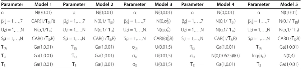
Parameter Model 1 Parameter Model 2 Parameter Model 3 Parameter Model 4 Parameter Model 5
α N(0,0.01) α N(0,0.01) α N(0,0.01) α N(0,0.01) α N(0,0.01)
βj;j = 1,…,7 CAR(1/Ƭβj,R) βj;j = 1,…,7 N(0,1/Ƭβj) βj;j = 1,…,7 N(0,σ 2
βj) βj;j = 1,…,7 N(0,1/Ƭβj) βj;j = 1,…,7 N(0,1/Ƭβj) Ui;i = 1,…,N N(α,1/ƬU) Ui;i = 1,…,N N(α,1/ƬU) Ui;i = 1,…,N N(α,σ2U) Ui;i = 1,…,N N(α,1/ƬU) Ui;i = 1,…,N N(α,1/ƬU) Si;i = 1,…,N CAR(1/ƬS,R) Si;i = 1,…,N CAR(1/ƬS,R) Si;i = 1,…,N CAR((σ2S,R) Si;i = 1,…,N CAR(1/ƬS,R) Si;i = 1,…,N CAR(1/ƬS,R)
Ƭβj Ga(1,0.01) Ƭβj Ga(1,0.01) σβj U(0.01,5) Ƭβj Ga(1,0.01) Ƭβj Ga(1,0.01)
ƬU Ga(1,0.01) ƬU Ga(1,0.01) σU U(0.01,5) σU N(0,0.0625)I(0,) log(σU) N(0,4)
ƬS Ga(1,0.01) ƬS Ga(1,0.01) σS U(0.01,5) ƬS Ga(1,0.01) ƬS Ga(1,0.01)
α= intercept, j = covariates 1 to 7,βj= vector of coefficients for covariates 1 to 7, i = Local Government Areas (LGAs) 1 to 71, Ui= uncorrelated residual error for
LGAs 1 to 71, Si= correlated residual error for LGAs 1 to 71,Ƭβj= vector of precisions for covariate coefficients,ƬU= vector of precisions for uncorrelated residual
error,ƬS= vector of precisions for correlated residual error,σβj= vector of standard deviations for covariate coefficients,σU= vector of standard deviations for
uncorrelated residual error,σS= vector of standard deviations for correlated residual error, Ga = Gamma distribution, U = Uniform distribution, CAR = CAR normal
prior centred around zero, denoted CAR(variance, adjacency neighbourhood weight matrix), R = adjacency neighbourhood weight matrix with diagonal entries equal to number of neighbours; ie.Rii=mi.
Table 2 Comparison of imputation methods by root mean squared error (RMSE) and bias from cross-validation
Covariate N
missing
RMSE, mean (sd) Average bias
Average width of CI
% of CIs including zero
bias Mean
imputation
MVN CAR prior
Poisson Binomial Poisson Binomial MVN CAR prior
MVN CAR prior
MVN CAR prior
% over 45yrs of age 3 49.7 108.7 (21.2) 109.6 (19.5) 46.3 (17.8) 46.2 (17.9) 0.012 0.041 0.897 0.345 100% 100% % Overweight/obese 28 26.3 73.7 (22.3) 73.1 (20.6) 45.4 (18.5) 45.4 (18.4) 0.016 0.081 0.413 0.200 100% 75% % Daily smokers 28 25.8 53.2 (18.1) 54.4 (19.3) 49.8 (21.1) 49.8 (21.0) 0.153 0.271 1.144 0.640 100% 68% % Insufficient physical
activity
28 36.7 90.7 (37.5) 91.4 (37.1) 67.0 (41.3) 67.1 (41.3) 0.048 0.047 0.535 0.246 100% 93%
% Adequate fruit intake 28 34.4 67.4 (14.3) 68.6 (14.7) 37.5 (22.7) 37.6 (22.7) 0.069 0.052 0.382 0.221 100% 91% % Adequate vegetable
intake
32 21.9 39.1 (18.5) 39.2 (18.4) 30.4 (19.6) 30.6 (19.9) 0.157 0.185 1.144 0.973 100% 94%
Overall - 32.5 71.1 (11.4) 72.7 (11.1) 46.1 (11.7) 46.1 (11.7) 0.076 0.113 0.752 0.438 100% 87%
displayed in Table 3. Each of the GLMMs included in sensitivity analysis produced similar coefficient estimates and resulted in the same conclusions.
Results
SES was found to be the only variable associated with DM II RR based on the Poisson models and prevalence based on the Binomial models, from both univariate and multi-variate models. Of the other comulti-variates included in the models, none were found to be significantly associated with DM II outcomes. From the baseline Poisson model (model 1), each one unit increase in SES was estimated to decrease the log(relative risk) of DM II by 0.18 (95% cred-ible interval 0.13 to 0.23).
Mediation analysis did not find a significant mediating effect (defined by a change of 10% or more to the SES coefficient) between SES and DM II RR by any of the other covariates included in this study.
Geographic variation
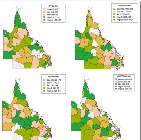
Spatially smoothed relative risks (RR) and relative excess risks (RER) and corresponding standard deviations and 95% credible intervals were obtained from the Poisson GLMMs with mean imputation and CAR priors fit to covariate data. The estimated RR of DM II varied be-tween study regions from 0.48 (Isaac Regional) to 3.07 (Cherbourg Aboriginal Shire), indicating a six-fold vari-ation (3.07/0.48 = 6.4) across regions. RER varied from 0.96 for Napranum Aboriginal Shire to 4.44 for Burke Shire. The distribution of RR and RER by quintiles from
highest to lowest are displayed in Figure 2 along with their standard deviation. The size of estimated RR and RER for each region does not appear to be associated with the size of uncertainty for those regions.
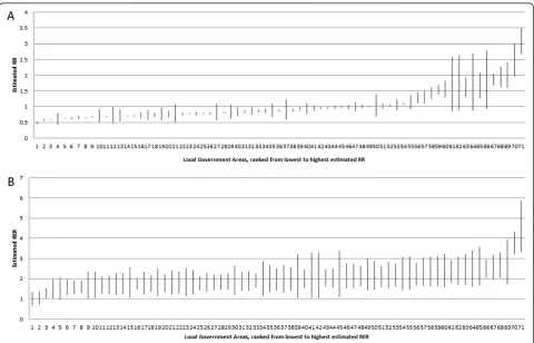
The LGAs with the five smallest and five highest RR, RER and standard deviation for RR and RER are ranked in Table 4. 80% of the regions in the top five for large RR also were in the top five for large RER, indicating that they are most at risk for DM II occurrence even after accounting for the influence of regional risk factors.
Figure 3 ranks regions in order of low to high RR (A) and RER (B) respectively with 95% CIs. As may be ex-pected, regions with missing covariate data tended to have wider 95% CIs compared with regions with observed data.
Discussion
Our study describes an evaluation of three different im-putation methods that are applicable to missing health survey data for spatial analysis. Choice of imputation method depends upon the particular application and is not necessarily the most complex method. In the application for this case study, simple imputation with the mean value of each missing covariate value was found to provide the most accurate prediction of missing values in this dataset, based on the statistical measures described.
In this application, mean imputation was found to be more appropriate than imputation with CAR priors using spatial correlation of covariate data to impute missing values. For this dataset, this could be due to the large proportion of missingness for some covariates Figure 1Bias for estimated % over 45 years for Local Government Areas (LGAs) with missing data, by 1. Multivariate normal
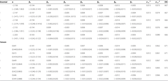
Table 3 Estimates for selected parameters from models included in sensitivity analysis: mean (95% credible intervals)
Binomial α β1 β2 β3 β4 β5 β6 β7 σS
2 σU
2
DIC
1 −2.158 −0.194 0.009 −0.004 0.008 −0.008 −0.013 −0.005 0.013 0.073 667
(−2.368,-1.963) (−0.240,-0.143) (−0.001,0.020) (−0.019,0.012) (−0.010,0.027) (−0.022,0.006) (−0.036,0.011) (−0.033,0.022)
2 −2.147 −0.197 0.009 −0.005 0.008 −0.007 −0.015 −0.004 0.013 0.074 667
(−2.415,-1.911) (−0.253,-0.129) (−0..002,0.021) (−0.024, 0.013) (−0.013, 0.027) (−0.023, 0.008) (−0.040,0.008) (−0.031,0.025)
3 −2.158 −0.194 0.01 −0.005 0.008 −0.007 −0.014 −0.005 0.012 0.079 666
(−2.374,-1.939) (−0.248,-0.1416) (−0.002,0.021) (−0.022,0.011) (−0.010,0.026) (−0.022,0.006) (−0.038,0.007) (−0.032,0.022)
4 −2.155 −0.194 0.009 −0.003 0.008 −0.007 −0.014 −0.004 0.012 0.076 668
(−2.384,-1.951) (−0.242,-0.138) (−0.002,0.0196) (−0.020,0.016) (−0.010,0.026) (−0.022,0.008) (−0.038,0.009) (−0.030,0.023)
5 −2.203 −0.183 0.008 −0.004 0.008 −0.006 −0.013 −0.003 0.012 0.080 666
(−2.451,-1.953) (−0.242,-0.122) (−0.004,0.020) (−0.026,0.015) (−0.013,0.029) (−0.024,0.011) (−0.037,0.009) (−0.032,0.027)
Poisson
1 0.641 −0.181 0.009 −0.005 0.007 −0.006 −0.014 −0.005 0.012 0.062 671
(0.440,0.854) (−0.232,-0.134) (−0.001,0.020) (−0.022,0.011) (−0.009,0.024) (−0.020,0.008) (−0.035,0.008) (−0.030,0.022)
2 0.615 −0.174 0.008 −0.004 0.008 −0.005 −0.011 −0.004 0.012 0.061 671
(0.434,0.816) (−0.223,-0.133) (−0.002,0.018) (−0.020,0.012) (−0.008,0.026) (−0.018,0.007) (−0.031,0.009) (−0.028,0.022)
3 0.649 −0.183 0.009 −0.004 0.008 −0.006 −0.013 −0.003 0.012 0.067 670
(0.413,0.864) (−0.236,-0.125) (−0.002,0.020) (−0.025,0.014) (−0.010,0.025) (−0.021,0.008) (−0.036,0.011) (−0.029,0.025)
4 0.651 −0.184 0.009 −0.004 0.007 −0.007 −0.013 −0.005 0.012 0.065 672
(0.422,0.883) (−0.240,-0.129) (−0.002,0.020) (−0.023,0.014) (−0.012,0.025) (−0.021,0.007) (−0.036,0.010) (−0.031,0.022)
5 0.646 −0.182 0.009 −0.003 0.008 −0.007 −0.012 −0.006 0.011 0.066 670
(0.441,0.888) (−0.244,-0.134) (−0.002,0.020) (−0.021,0.016) (−0.012,0.025) (−0.022,0.008) (−0.034,0.009) (−0.030,0.022)
α= intercept,β1= coefficient for socio-economic status,β2= coefficient for % over 45 years of age,β3= coefficient for % overweight/obese,β4= coefficient for % daily smokers,β5= coefficient for % insufficient physical
activity,β6= coefficient for % adequate fruit intake,β7= coefficient for % adequate vegetable intake,σS2= variance of correlated residual error,σU2= variance of uncorrelated residual error,DIC= Deviance
Information Criteria.
Prior distributions used in models 1–5 are summarised in Table1.
Interna
tional
Journal
of
Health
Geographics
2014,
13
:47
Page
9
o
f
1
3
graphics.co
m/content/13/1
relative to a small number of neighbours for certain re-gions, providing insufficient observed data from neigh-bouring regions. These different imputation methods may perform comparatively differently in datasets with smaller proportions of missing data.
Simple mean imputation was also found to be far more accurate in this case study than fitting a multivari-ate normal distribution to covarimultivari-ates to impute missing data in this dataset, despite empirical evidence of high
status survey. Thus data were not missing at random in this dataset. Multivariate normal imputation may provide more accurate prediction of missing values in datasets with missingness at random as well as high correlations between covariate pairs.
Our sensitivity analysis provides evidence that choice of priors, from non-informative to more informative choices, did not affect results from the spatial analysis of this case study. Fitting of Binomial and Poisson models produced similar findings with similar goodness of fit as measured by
Table 4 Top 5 LGAs for Relative Risk (RR), Relative Excess Risk (RER) and uncertainty for Relative Risk and Excess Relative Risk
Smallest estimated RR Smallest sd(RR) Smallest estimated RER Smallest sd (RER)
LGA Estimated RR LGA sd(RR) LGA Estimated ERR LGA sd(RER)
34 0.480 8 0.003 47 0.962 67 0.125
16 0.573 28 0.005 32 1.021 10 0.150
8 0.580 44 0.006 67 1.255 30 0.152
24 0.611 60 0.006 34 1.442 32 0.161
28 0.624 38 0.007 24 1.452 57 0.168
Largest estimated RR Largest sd(RR) Largest estimated RER Largest sd(RER)
LGA LGA sd(RR) LGA Estimated RER LGA sd(RER)
63 1.857 12 0.269 51 2.535 68 0.566
35 1.933 41 0.445 35 2.627 70 0.575
51 1.966 65 0.452 68 2.645 41 0.580
12 2.450 70 0.465 18 3.738 23 0.587
18 3.073 23 0.474 12 4.442 12 0.647
RR= Relative Risk,RER= Relative Excess Risk,sd= standard deviation.
DIC. This supports the estimates of DM II RR for each LGA and evidence that SES is strongly associated with DM II risk in this region. The sensitivity analysis described in this paper is readily applicable to spatial analysis of other health datasets.
Several studies have examined geographic variation in DM II in the US, UK and Europe, however, less is known about regional variation and associated regional risk factors in Australia. Similar to other studies, our analysis shows marked geographic variation in DM II relative risk [7,9,11-18]. Just within Queensland, our study estimates a six-fold difference in DM II relative risk. Similar to findings from other spatial studies, we found lower socioeconomic status to be strongly associated with increased risk of DM II [9,11,13,14].
Contrary to findings from Green et al., we did not find the proportion of daily smokers to be associated with DM II risk [11]. In comparison with risk models reporting BMI to be associated with DM II risk at an individual-level, we did not find the proportion of residents overweight or obese to be associated with DM II risk at a regional level in this dataset [8]. We examined the association of obesity (BMI≥30kg/m2) and overweight (25kg/m2≤BMI < 30kg/m2) with DM II RR separately in univariate models and neither were found to be significant within this geographic region. However, our study categorised BMI into broad overweight and obese categories whereas the risk models considered raw BMI scores. Findings may differ for spatial analyses of DM II risk in other regions.
Strengths of our study include that we were able to evaluate the performance of three different imputation approaches using methodology which is immediately applicable to other regions and health datasets outside the application of the case study reported. Within our case study, we were able to evaluate the geographical vari-ation in DM II RR across Queensland and identify re-gions of high risk, and regional factors associated with DM II risk, accounting for missing data. We used Bayesian methods to fit hierarchical models accounting for different sources of uncertainty, to evaluate the as-sociation of geographical covariates with DM II RR. Spatial smoothing was performed, accounting for cor-relation between neighbouring regions and mitigating the effects of random measurement error. In addition, we were able to select the most accurate imputation method for this dataset and check the accuracy of results through sensitivity analysis.
Limitations of our study include the presence of sig-nificant missing data, small sample sizes for test datasets in cross-validation, that diabetic counts were based on notification data with unknown measurement bias, and that region-level lifestyle data was based on self-report that is not objectively measured. Thus results should be interpreted with caution.
Although spatial modelling of DM II relative risk at a smaller region level such as Statistical Local Area (SLA) may have resulted in relative risk information at a finer level, the difficulty is that lifestyle information is not avail-able at this level and cannot be assessed for contribution to DM II risk. Furthermore, we expect less uncertainty from variation in notification rates when data is aggregated to a larger regional level.
Conclusions
In conclusion, we present a method for selection of an ap-propriate imputation method among alternative choices suited to spatial health survey data with varying patterns and amounts of missingness. Missing data is a common problem with spatial health data, and appropriate choice of imputation method depends upon the particular appli-cation. As discovered for the case study considered here, choice of imputation method may not always be the most complex one. However in some cases, utilising other information such as spatial correlation in data or correl-ation between covariates may be appropriate for the pur-poses of imputation. Selection of an appropriate imputation method allows a more complete analysis of geographic risk factors for disease at a regional level, with the potential to inform resource allocation and public policy, and reduce the burden of disease to the community.
This case study provides evidence of a six-fold differ-ence in geographical variation in DM II RR across Queensland LGAs, and indicates that socio-economic status is strongly associated with DM II risk. Our results indicate that a geographically targeted approach to managing DM II may be effective, and highlight regions most in need of additional services to manage DM II. The methodology used in this study is applicable to spatial analyses of diabetes in other regions, as well as other diseases, and has the potential to provide useful informa-tion for management and resource allocainforma-tion decisions.
Additional file
Additional file 1:Bias for estimates for each covariate for regions with missing data.
Competing interests
The authors declare that they have no competing interests.
Authors’contributions
JB, NW and KM contributed to the concept and design of this study. JB was involved in the acquisition, analysis and interpretation of the data and drafting of the manuscript. All authors contributed to revision of the manuscript and approved the final manuscript.
Acknowledgements
Received: 29 August 2014 Accepted: 10 November 2014 Published: 20 November 2014
References
1. Earnest A, Morgan G, Mengersen KL, Ryan L, Summerhayes R, Beard J: Evaluating the effect of neighbourhood weight matrices on smoothing properties of Conditional Autoregressive (CAR) models.Int J Health Geogr
2007,6:54.
2. Besag J, York J, Mollie A:Bayesian image restoration with two application in spatial statistics.Annc Inst Statist Math1991,43(1):1–59.
3. Diabetes UK:Diabetes in the UK 2012.Diabetes UK2012, [http://www. diabetes.org.uk/Documents/Reports/Diabetes-in-the-UK-2012.pdf] 4. Holden SH, Barnett AH, Peters JR, Jenkins-Jones S, Poole CD, Morgan CL,
Currie CJ:The incidence of type 2 diabetes in the United Kingdom from 1991 to 2010.Diabetes Obes Metab2010,15(9):844–852.
5. Palmer AJ, Tucker DM:Cost and clinical implications of diabetes prevention in an Australian setting: a long-term modeling analysis.
Prim Care Diabetes2012,6(2):109–121.
6. Harris MI, Eastman RC:Early detection of undiagnosed diabetes mellitus: a US perspective.Diabetes Metab Res Rev2000,16(4):230–236.
7. Liese AD, Lawson A, Song HR, Hibbert JD, Porter DE, Nichols M, Lamichhane AP, Dabelea D, Mayer-Davis EJ, Standiford D, Liu L, Hamman RF, D’Agostino RB Jr:Evaluating geographic variation in type 1 and type 2 diabetes mellitus incidence in youth in four US regions.Health Place2010,16(3):547–556. 8. Noble D, Mathur R, Dent T, Meads C, Greenhalgh T:Risk models and scores
for type 2 diabetes: systematic review.BMJ2011,343:d7163. 9. Weng C, Coppini DV, Sonksen PH:Geographic and social factors are
related to increased morbidity and mortality rates in diabetic patients.
Diabet Med2000,17(8):612–617.
10. Egede LE, Gebregziabher M, Hunt KJ, Axon RN, Echols C, Gilbert GE, Mauldin PD:Regional, geographic, and racial/ethnic variation in glycemic control in a national sample of veterans with diabetes.Diabetes Care2011, 34(4):938–943.
11. Green C, Hoppa RD, Young TK, Blanchard JF:Geographic analysis of diabetes prevalence in an urban area.Soc Sci Med2003,57(3):551–560. 12. Bocquier A, Cortaredona S, Nauleau S, Jardin M, Verger P:Prevalence of
treated diabetes: Geographical variations at the small-area level and their association with area-level characteristics. A multilevel analysis in Southeastern France.Diabetes Metab2011,37(1):39–46.
13. Geraghty EM, Balsbaugh T, Nuovo J, Tandon S:Using Geographic Information Systems (GIS) to assess outcome disparities in patients with type 2 diabetes and hyperlipidemia.J Am Board Fam Med2010, 23(1):88–96. Jan-Feb.
14. Chaix B, Billaudeau N, Thomas F, Havard S, Evans D, Kestens Y, Bean K: Neighborhood effects on health: correcting bias from neighborhood effects on participation.Epidemiology2011,22(1):18–26.
15. Congdon P:Estimating diabetes prevalence by small area in England.
J Public Health (Oxf )2006,28(1):71–81.
16. Kravchenko VI, Tronko ND, Pankiv VI, Venzilovich Yu M, Prudius FG: Prevalence of diabetes mellitus and its complications in the Ukraine.
Diabetes Res Clin Pract1996,34(Suppl):S73–S78.
17. Lee JM, Davis MM, Menon RK, Freed GL:Geographic distribution of childhood diabetes and obesity relative to the supply of pediatric endocrinologists in the United States.J Pediatr2008,152(3):331–336. 18. Noble D, Smith D, Mathur R, Robson J, Greenhalgh T:Feasibility study of
geospatial mapping of chronic disease risk to inform public health commissioning.BMJ Open2012,2(1):e000711.
19. Magalhaes RJ, Clements AC:Mapping the risk of anaemia in preschool-age children: the contribution of malnutrition, malaria, and helminth infections in West Africa.PLoS Med2011,8(6):e1000438.
20. Stromberg U, Magnusson K, Holmen A, Twetman S:Geo-mapping of caries risk in children and adolescents - a novel approach for allocation of preventive care.BMC Oral Health2011,11:26.
21. Joshua V, Gupte MD, Bhagavandas M:A Bayesian approach to study the space time variation of leprosy in an endemic area of Tamil Nadu, South India.Int J Health Geogr2008,7:40.
22. Cocco E, Sardu C, Massa R, Mamusa E, Musu L, Ferrigno P, Melis M, Montomoli C, Ferretti V, Coghe G, Fenu G, Frau J, Lorefice L, Carboni N, Contu P, Marrosu MG:Epidemiology of multiple sclerosis in south-western Sardinia.Mult Scler2011,17(11):1282–1289.
23. Goovaerts P:Geostatistical analysis of disease data: accounting for spatial support and population density in the isopleth mapping of cancer mortality risk using area-to-point Poisson kriging.Int J Health Geogr2006,5:52. 24. Hegarty AC, Carsin AE, Comber H:Geographical analysis of cancer
incidence in Ireland: a comparison of two Bayesian spatial models.
Cancer Epidemiol2010,34(4):373–381.
25. Cramb SM, Mengersen KL, Baade PD:Developing the atlas of cancer in Queensland: methodological issues.Int J Health Geogr2011,10:9. 26. Haque U, Magalhaes RJ, Reid HL, Clements AC, Ahmed SM, Islam A,
Yamamoto T, Haque R, Glass GE:Spatial prediction of malaria prevalence in an endemic area of Bangladesh.Malar J2010,9:120.
27. Zayeri F, Salehi M, Pirhosseini H:Geographical mapping and Bayesian spatial modeling of malaria incidence in Sistan and Baluchistan province, Iran.Asian Pac J Trop Med2011,4(12):985–992. 28. Stensgaard AS, Vounatsou P, Onapa AW, Simonsen PE, Pedersen EM,
Rahbek C, Kristensen TK:Bayesian geostatistical modelling of malaria and lymphatic filariasis infections in Uganda: predictors of risk and geographical patterns of co-endemicity.Malar J2011,10:298. 29. Kang SY, McGree J, Mengersen K:The impact of spatial scales and spatial
smoothing on the outcome of bayesian spatial model.PLoS One2013, 8(10):e75957.
30. National Diabetes Services Scheme:Australian Diabetes Map.2012 [www.ndss.com.au/Australian-Diabetes-Map/]
31. Australian Bureau of Statistics:3218.0 Population Estimates by Local Government Area, 2001 to 2011.2012, [www.abs.gov.au/AUSSTATS/abs@. nsf/DetailsPage/3218.02011]
32. Queensland Government:Queensland self-reported health status 2009–2010: Local Government Area summary report.2011 [http://www.health.qld.gov.au/ epidemiology/documents/srhs0910lgasummary.pdf]
33. Besag J:Spatial interaction and the statistical analysis of lattice systems.
J Royal Sta Soc Ser B (Methodological)1974,36(2):192–236.
34. Pascutto C, Wakefield JC, Best NG, Richardson S, Bernardinelli L, Staines A, Elliott P:Statistical issues in the analysis of disease mapping data.Stat Med2000,19(17–18):2493–519. Sep 15–30.
35. The R Project:The R Project for Statistical Computing.2014 [ http://www.r-project.org/] 36. The BUGS Project:WinBUGS.2014 [http://www.mrc-bsu.cam.ac.uk/software/
bugs/the-bugs-project-winbugs/]
37. Spiegelhalter D, Best NG, Carlin B, Van Der Linde A:Bayesian measures of model complexity and fit.J Royal Sta Soc2002,64(4):583–639.
doi:10.1186/1476-072X-13-47
Cite this article as:Bakeret al.:Missing in space: an evaluation of imputation methods for missing data in spatial analysis of risk factors for type II diabetes.International Journal of Health Geographics201413:47.
Submit your next manuscript to BioMed Central and take full advantage of:
• Convenient online submission
• Thorough peer review
• No space constraints or color figure charges
• Immediate publication on acceptance
• Inclusion in PubMed, CAS, Scopus and Google Scholar
• Research which is freely available for redistribution