The Thirty-Third AAAI Conference on Artificial Intelligence (AAAI-19)
Online Embedding Compression for Text
Classification Using Low Rank Matrix Factorization
Anish Acharya,
∗1Rahul Goel,
1Angeliki Metallinou,
1Inderjit Dhillon
2,3 1Amazon Alexa AI,2Amazon Search Technologies,3University of Texas at Austin{achanish, goerahul, ametalli}@amazon.com, [email protected]
Abstract
Deep learning models have become state of the art for nat-ural language processing (NLP) tasks, however deploying these models in production system poses significant memory constraints. Existing compression methods are either lossy or introduce significant latency. We propose a compression method that leverages low rank matrix factorization during training, to compress the word embedding layer which rep-resents the size bottleneck for most NLP models. Our mod-els are trained, compressed and then further re-trained on the downstream task to recover accuracy while maintaining the reduced size. Empirically, we show that the proposed method can achieve 90% compression with minimal impact in accu-racy for sentence classification tasks, and outperforms alter-native methods like fixed-point quantization or offline word embedding compression. We also analyze the inference time and storage space for our method through FLOP calcula-tions, showing that we can compress DNN models by a con-figurable ratio and regain accuracy loss without introducing additional latency compared to fixed point quantization. Fi-nally, we introduce a novel learning rate schedule, the Cycli-cally Annealed Learning Rate (CALR), which we empiriCycli-cally demonstrate to outperform other popular adaptive learning rate algorithms on a sentence classification benchmark.
1
Introduction
Deep learning has achieved great success in various NLP tasks such as sequence tagging (Chung et al. 2014), (Ma and Hovy 2016) and sentence classification (Liu et al. 2015; Kim 2014). While traditional machine learning approaches extract hand-designed and task-specific features, which are fed into a shallow model, neural models pass the input through several feedforward, recurrent or convolutional lay-ers of feature extraction that are trained to learn automatic feature representations. However, deep neural models of-ten have large memory-footprint and this poses significant deployment challenges for real-time systems that typically have memory and computing power constraints. For exam-ple, mobile devices tend to be limited by their CPU speed, memory and battery life, which poses significant size con-straints for models embedded on such devices. Similarly,
∗
Corresponding Author
Copyright c2019, Association for the Advancement of Artificial Intelligence (www.aaai.org). All rights reserved.
models deployed on servers need to serve millions of re-quests per day, therefore compressing them would result in memory and inference cost savings.
For NLP specific tasks, the word embedding matrix often accounts for most of the network size. The embedding ma-trix is typically initialized with pretrained word embeddings like Word2Vec, (Mikolov et al. 2013) FastText (Bojanowski et al. 2016) or Glove (Pennington, Socher, and Manning 2014) and then fine-tuned on the downstream tasks, includ-ing tagginclud-ing, classification and others. Typically, word em-bedding vectors are 300-dimensional and vocabulary sizes for practical applications could be up to 1 million tokens. This corresponds to up to 2Gbs of memory and could be prohibitively expensive depending on the application. For example, to represent a vocabulary of 100K words using 300 dimensional Glove embeddings the embedding matrix would have to hold 60M parameters. Even for a simple sen-timent analysis model the embedding parameters are 98.8% of the total network (Shu and Nakayama 2017).
In this work, we address neural model compression in the context of text classification by applying low rank matrix factorization on the word embedding layer and then re-training the model in an online fashion. There has been rel-atively less work in compressing word embedding matrices of deepNLP models. Most of the prior work compress the embedding matrix offline outside the training loop either through hashing or quantization based approaches (Joulin et al. 2016; Shu and Nakayama 2017; Raunak 2017).
Our approach includes starting from a model initialized with large embedding space, performing a low rank pro-jection of the embedding layer using Singular Value De-composition (SVD) and continuing training to regain any lost accuracy. This enables us to compress a deep NLP model by an arbitrary compression fraction (p), which can be pre-decided based on the downstream application con-straints and accuracy-memory trade-offs. Standard quantiza-tion techniques do not offer this flexibility, as they typically allow compression fractions of1/2or1/4(corresponding to 16-bit or 8-bit quantization from 32-bits typically).
outper-forms popular compression techniques including quantiza-tion (Hubara et al. 2016) and offline word embedding size reduction (Raunak 2017).
A second contribution of this paper is the introduction of a novel learning rate schedule,we call Cyclically Annealed Learning Rate (CALR), which extends previous works on cyclic learning rate (Smith 2017) and random hyperparame-ter search (Bergstra and Bengio 2012). Our experiments on SST2 demonstrate that for both DAN (Iyyer et al. 2015) and LSTM (Hochreiter and Schmidhuber 1997) models CALR outperforms the current state-of-the-art results that are typi-cally trained using popular adaptive learning like AdaGrad. Overall, our contributions are:
• We propose a compression method for deep NLP mod-els that reduces the memory footprint through low rank matrix factorization of the embedding layer and regains accuracy through further finetuning.
• We empirically show that our method outperforms popu-lar baselines like fixed-point quantization and offline em-bedding compression for sentence classification.
• We provide an analysis of inference time for our method, showing that we can compress models by an arbitrary configurable ratio, without introducing additional latency compared to quantization methods.
• We introduce CALR, a novel learning rate scheduling al-gorithm for gradient descent based optimization and show that it outperforms other popular adaptive learning rate al-gorithms on sentence classification.
2
Related Work
In recent literature, training overcomplete respresentations is often advocated as overcomplete bases can transform local minima into saddle points (Dauphin et al. 2014) or help dis-cover robust solutions (Lewicki and Sejnowski 2000). This indicates that significant model compression is often possi-ble without sacrificing accuracy and that the model’s accu-racy does not rely on precise weight values (Keskar et al. 2016). Most of the recent work on model compression ex-ploits this inherent sparsity of overcomplete represantations. These works include low precision computations (Anwar, Hwang, and Sung 2015; Courbariaux, Bengio, and David 2014) and quantization of model weights (Han, Mao, and Dally 2015; Zhou et al. 2017). There are also methods which prune the network by dropping connections with low weights (Wen et al. 2016; See, Luong, and Manning 2016) or use sparse encoding (Han et al. 2015). These methods in practice often suffer from quantization loss especially if the network is deep due to a large number of low-precision mul-tiplications during forward pass. Quantization loss is hard to recover through further training due to the non-trivial na-ture of backpropagation in low precision (Lin et al. 2015). There has been some work on compression aware train-ing (Polino, Pascanu, and Alistarh 2018) via model distil-lation (Hinton, Vinyals, and Dean 2015) that addresses this gap in accuracy. However, both quantized distillation and differentiable quantization methods introduce additional la-tency due to their slow training process that requires careful tuning, and may not be a good fit for practical systems where a compressed model needs to be rapidly tuned and deployed
in production.
Low-rank matrix factorization (LMF) is a very old dimen-sionality reduction technique widely used in the matrix com-pletion literature (see (Recht and R´e 2013) and references therein). However, there has been relatively limited work on applying LMF to deep neural models. (Sainath et al. 2013; Lu, Sindhwani, and Sainath 2016) used low rank matrix fac-torization for neural speech models.While (Sainath et al. 2013) reduces parameters of DNN before training, (Xue, Li, and Gong 2013) restructures the network using SVD intro-ducing bottleneck layers in the weight matrices. However, for typical NLP tasks, introducing bottleneck layers between the deep layers of the model does not significantly decrease model size since the large majority of the parameters in NLP models come from the input word embedding matrix. Build-ing upon this prior work, we apply LMF based ideas to re-duce the embedding space of NLP models. Instead of ex-ploiting the sparsity of parameter space we argue that for overcomplete representation the input embedding matrix is not a unique combination of basis vectors (Lewicki and Se-jnowski 2000). Thus, it is possible to find a lower dimen-sional parameter space which can represent the model in-puts with minimal information loss. Based on this intuition, we apply LMF techniques for compressing the word embed-ding matrix which is the size bottleneck for many NLP tasks.
3
Methodology
3.1
Low-rank Matrix Factorization (LMF) for
Compressing Neural Models
Low-rank Matrix Factorization (LMF) exploits latent struc-ture in the data to obtain a compressed representation of a matrix. It does so by factorization of the original matrix into low-rank matrices. For a full rank matrix W ∈ Rm×n of
rankr, there always exists a factorizationW = Wa×Wb
whereWa ∈ Rm×randWb ∈ Rr×n. Singular Value De-composition (SVD) (Golub and Reinsch 1970) achieves this factorization as follows:
Wm×n=Um×mΣm×nVnt×n (1)
where Σm×n is a diagonal rectangular matrix of singular
values of descending magnitude. We can compress the ma-trix by choosing theklargest singular values, withk < m
andk < n. For low rank matrices, the discarded singular values will be zero or small, therefore the following will ap-proximately hold:
Wm×n≈Um×kΣk×kVkt×n (2)
Therefore, the original matrixW is compressed into two matrices:
Wa=U ∈Rm×k (3)
Wb= Σk×kVkt×n∈R
k×n (4)
The number of parameters are reduced from m×nto
k×(m+n). Therefore, to achieve apfraction parameter reduction,kshould be selected as:
(p×m×n) =k×(m+n)
k=
pmn
m+n
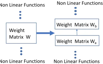
The valuekcan be varied depending on the desired com-pression fractionpas long ask≥1. In practice, being able to decide an arbitrary compression fractionpis an attractive property for model compression, since it allows choosing compression rates based on the accuracy-memory trade-offs of a downstream application. The low rank matrix factoriza-tion operafactoriza-tion is illustrated in Figure 1, where a single neural network matrix (layer) is replaced by two low rank matrices (layers).
Figure 1: Replacing one neural network matrix with two low rank matrices
Compressing the Word Embedding Matrix For NLP tasks, typically the first layer of the neural model consists of an embedding lookup layer that maps the words into real-valued vectors for processing by subsequent layers. The words are indicesiof a word dictionary of sizeDwhile the word embeddings are vectors of sized. This corresponds to a lookup table E(i) = Wi where W ∈ Rd×|D|. The word embeddings are often trained offline on a much larger corpus, using algorithms like Word2Vec, GloVe etc, and are then fine-tuned during training on the downstream NLP task. Our method decomposes the embedding layer in an online fashion during training using eq.(5).Wa becomes the new
embedding layer and Wb becomes the next layer.
Contin-uing backpropagation over this new network struture fine-tunes the low rank embedding space and regains any accu-racy loss within a few epochs.
3.2
Cyclically Annealed Learning Rate
Due to the non-convex nature of the optimization surface of DNNs, gradient based algorithms like stochastic gradient descent (SGD) are prone to getting trapped in suboptimal local minima or saddle points. Adaptive learning rates like Adam (Kingma and Ba 2014) and Adagrad (Duchi, Hazan, and Singer 2011) try to solve this problem by tuning learn-ing rate based on the magnitude of gradients. While in most cases they find a reasonably good solution, they usually can’t explore the entire gradient landscape. (Bergstra and Bengio 2012; Loshchilov and Hutter 2016) indicates periodic ran-dom initialization or warm restarts often helps in better ex-ploration of the landscape while (Smith 2017) showed that letting the learning rate(LR) vary cyclicaly (Cyclic learn-ing rate(CLR)) helps in faster convergence. In this work we further refine CLR and propose a simulated annealing in-spired LR update policy we call Cyclically Annealed Learn-ing Rate (CALR). CALR is described in algorithm (1) and
Fig. 2b. In addition to varying LR in a CLR style triangular windows(Fig. 2a), CALR expontentially decays the upper boundLRU Bof the triangular window from its initial value.
When the learning rate decreases to a lower boundLRLB,
we increase the upper bound to its initial valueLRU B and
continue with the LR updates. This exponential decay en-sures slow steps on the optimization landscape. Intuitively, the proposed warm restarts, motivated by simulated anneal-ing, make CALR more likely to escape from local minima or saddle points and enables better exploration of the parameter space. CALR should have similar but less aggressive effect as random initialization or warm restarts of LR. While expo-nentially decayed small cyclic windows let CALR carefully explore points local to the current solution, cyclic tempera-ture increase helps it jump out and explore regions around other nearby local minima. We verified this intuition em-pirically for our classification experiments (Table 1, Secton 5.4), where CALR was able to achieve further improvement compared to CLR and Adagrad.
(a) CLR (b) CALR
Figure 2: Comparison of CLR and CALR update Policy
Algorithm 1Cyclically Annealed Learning Rate Schedule
1: procedureCALR(Iteration, Step Size,LRLB,LRU B)
2: LRU B←LRU B(init)
3: LRLB←LRLB(init)
4: for eachEPOCHdo
5: LRU B ←LRU B×exp(Decay)
6: ifLRU B ≤LRLBthen
7: LRU B ←LRU B(init)
8: for eachTraining BATCHdo
9: LR←CLR(Iteration,StepSize,LRLB, LRU B)
returnLR
1: procedureCLR(Iteration, Step Size,LRLB,LRU B) . this procedure implements a triangular window of width StepSize and heightLRU B−LRLB
2: Bump←LRU B−LRLB StepSize
3: Cycle←(Iteration) mod (2×StepSize)
4: ifCycle < StepSizethen
5: LR←LRLB+ (Cycle×Bump)
6: else
7: LR←LRU B−(Cycle−StepSize)×Bump
returnLR
3.3
Baselines
Fixed Point Weight Quantization (Baseline 1) We com-pare our approach with widely used post-training fixed point quantization (Bengio, L´eonard, and Courville 2013; Gong et al. 2014) method where the weights are cast into a lower precision. This requires less memory to store them and doing low precision multiplications during forward propaga-tion improves inference latency.
Offline Embedding Compression (Baseline 2) In this set of baseline experiments we compress the embedding matrix in a similar way using SVD but we do it as a preprocess-ing step similar to (Raunak 2017; Joulin et al. 2016). For example, if we have a 300 dimensional embedding and we want a 90% parameter reduction we project it onto a 30 di-mensional embedding space and use this low didi-mensional embedding to train the NLP model.
4
Analysis
In this section we analyze space and latency trade-off in compressing deep models. We compare the inference time and storage space of floating point operations(FLOPs) be-tween our method and Baseline1(sec.3.3) on a 1-layer Neu-ral Network(NN) whose forward pass on input X can be rep-resented as:
f(X) =σ(XW) (6)
where X ∈ R1×m and W ∈ Rm×n and full rank. Our method reduces W into two low rank matricesWa andWb
converting (6) into two layer NN represented as:
f(X) =σ((X×Wa)×Wb) (7)
whereWa ∈Rm×kandWb ∈Rk×nare constructed as de-scribed in eq.(3) and eq.(4) choosing k as in eq.(5). Whereas, Baseline1 casts the elements ofW to lower precision with-out restructuring the network. Thus, the quantized represen-tation of a 1-layer NN is same as eq.(6) whereWiis cast to
a lower bit precision and eq. (7) is the corresponding repre-sentation in our approach whereWi remains in its original
precision.
4.1
Space Complexity Analysis
On Baseline1 each weight variable uses less number of bits for storage. Quantizing the network weights into low pre-cision, we achieve space reduction by a fraction BQ
BS where
BS bits are required to store a full precision weight andBQ
bits are needed to store low precision weight. In contrast, our approach described in section 3.1, achieves more space reduction as long as we choosek(from eq (5)) such that:
p < BQ BS
(8)
4.2
Time Complexity Analysis
Total number of FLOPs in multiplying two matrices (Tre-fethen and Bau III 1997) is given by:F LOP(A×B) = (2b−1)ac ∼ O(abc) whereA ∈ Ra×b,B ∈ Rb×c and AB∈Ra×c. Assuming one FLOP in a low precision matrix
operations takes TQ time and on a full precision matrix it
takesTS time, for the model structure given by eq. (6), we
have:a= 1, b=m, c =n. Hence, for the forward pass on a single data vectorX ∈R1×ma quantized model usesFQ
flops where:
FQ = (2m−1)n (9)
Our algorithm restructures the DNN given in eq. (6) into eq. (7) yieldingFS =FS1+FS2flops. where:
FS1= (2m−1)k, FS2= (2k−1)n
FS = 2(m+n)k−(n+k) (10)
The number of FLOPs in one forward pass our method would be less than that of in Baseline1 ifFQ< FSor
equiv-alently:
(2m−1)n >2(m+n)k−(n+k)
k < 2mn
2(m+n)−1 (11)
Under the reasonable assumption that 2(m+n) 1 or equivalently2(m+n)−1≈2(m+n), eq. (11) becomes:
k < mn
(m+n) (12)
Eq. (12) will hold as long as k in our method is chosen according to eq.(5) (since the fraction p is by definition
p < 1) However, guaranteeing less FLOPs does not guar-antee faster inference since quantized model requires less time per FLOP. Our method guarantees faster inference if the following condition holds:
FQTQ> FSTS
(2m−1)nTQ>[(2m−1)k+ (2k−1)n]TS
(2m−1)n
[(2m−1)k+ (2k−1)n] > TS TQ
(13)
whereTS andTQare time taken per FLOP for our method
and Baseline1 respectivly. Again, we can make the reason-able assumptions that 2m 1 and 2k 1, therefore
2m−1≈2metc. Then eq. (13) becomes:
mn (m+n)k >
TS TQ
(14)
Pluggingkfrom eq.(5) we have:
p < TQ TS
(15)
If we assume that the time per FLOP is proportional to the number of bits B for storing a weight variable, e.g.,
TQ ∼BQandTS ∼BS then selectingpsuch thatp < BBQ S
will ensure that eq. (15) holds. In most practical scenarios time saving is sublinear in space saving which means eq.(8) is necessary and sufficient to ensure our method has faster inference time than fixed point quantization(Baseline1).
5
Experiments and Results
5.1
Datasets:
For all the experiments reported we have used the following two sentence classification datasets:
Stanford Sentiment Treebank (SST2)SST2 (Socher et al. 2013) is a common text classification benchmark dataset that contains movie reviews, to be classified according to their sentiment. On an average the reviews are about 200 words long. The dataset contains standard train, dev, test splits and binary sentiment labels.
Books Intent Classification DatasetWe use a proprietary dataset of around 60k annotated utterances of users interact-ing with a popular digital assistant about books related func-tionality. Each utterance is manually labeled with the user intent e.g., search for a book, read a book and others, with the task being to predict the user intent from a set of 20 in-tents. We choose 50k utterances as our training data, 5k as test data and 5k as dev data.
5.2
Models:
We evaluate our compression strategy on two types of widely used neural models:
Long Short Term Memory(LSTM) LSTMs, are power-ful and popular sequential models for classification tasks. The LSTM units are recurrent inn nature, designed to han-dle long term dependencies through the use of input, out-put and forget gates and a memory cell. For inout-put X = x1,· · ·xT and corresponding word embedding input
vec-tors ei, i = 1,· · ·T, LSTM computes a representation rt
at each wordt, which is denoted asrt=φ(et, rt−1). Here,
for sentence classification, we used the representation ob-tained from the final timestep of the LSTM and pass it through a softmax for classification: rsent = rTf orw, and
ˆ
S =sof tmax(Wsrsent+bs)wherersent is the sentence
representation, andSˆ is the label predicted. In our experi-ments with LSTM, we used 300-dimensional Glove embed-dings to initialize the embedding layer for all the methods, e.g., baselines 1, 2 and our proposed compression method. Our vocabulary sizeV contains only the words that appear in the training data, and we compress the input word embed-ding matrixW (original sizeV ×300).
Deep Averaging Network (DAN)DAN is a bag-of-words neural model that averages the word embeddings in each in-put utterance to create a sentence representationrsent that
is passed through a series of fully connected layers, and fed into a softmax layer for classification. Assume an input sen-tenceX of lengthT and corresponding word embeddings
ei, then the sentence representation is:rsent =T1 P T i=1ei
In our setup, we have two fully connected layers after the sentence representationrsent, of sizes 1024 and 512 respec-tively. For the DAN experiments we used the DAN-RAND (Iyyer et al. 2015) variant where we take a randomly initial-ized 300 dimensional embedding. To make the comparison fair, all experiments with DAN models, including quantiza-tion (baseline 1), the offline compression method (baseline 2) and the proposed compression method are done using ran-domly initialized word embedding matrices. For example, our baseline 2 is to use appropriate low-rank randomly ini-tialized embedding matrix.
5.3
Experimental Setup
Our experiments are performed on 1 Tesla K80 GPU, using SGD optimizer with CALR policy (Sec.3.2), initial learning rate upper bound of 0.001. We use dropout of 0.4 between layers and L2 regularization with weight of 0.005. Our met-rics include accuracy and model size. Accuracy is simply the fraction of utterances with correctly predicted label. The model size is calculated as sum of (.data + .index + .meta) files stored by tensorflow.
5.4
Results on Uncompressed Models
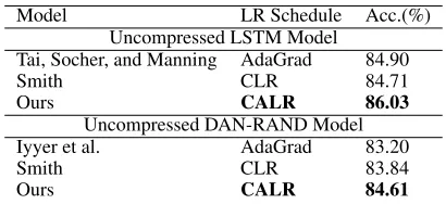
To effectively train our uncompressed benchmark networks we experimented with different adaptive learning rate sched-ules. Table 1 emperically demonstrates the effectiveness of our proposed learning rate update policy (CALR) on the SST2 test set. For both the models CALR outperforms the corresponding state-of-the-art sentence classification accu-racy reported in the literature. For LSTM we improve the accuracy from 84.9% (Socher et al. 2013) to 86.03% (1.33% relative improvement) whereas on DAN-RAND we are able to improve from 83.2% (Iyyer et al. 2015) to 84.61% (1.7% relative improvement). We also report results on training the network with CLR without our cyclic annealing. For both DAN-RAND and LSTM, CLR achieves performance that is similar to the previously reported state-of-the-art. The pro-posed CALR outperforms CLR, which supports the effec-tiveness of the proposed CALR policy.
5.5
Results on SST2
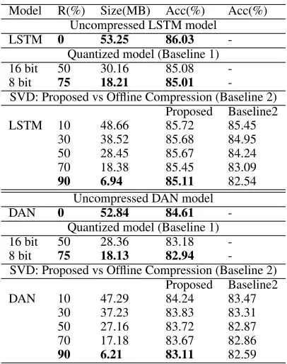
Table 2 shows compression and accuracy results on the SST2 test dataset for our proposed methods, the two base-lines described in Section 3.3, and for two types of mod-els: LSTM (upper table rows) and DAN-RAND (lower table rows). For both types of models, we first report the original uncompressed model size and accuracy. For the quantization baseline (baseline 1), we report size and accuracy numbers for 8-bit and 16-bit quantization. For the SVD-based meth-ods, both for the offline embedding compression (baseline 2) and our proposed compression method, we compare size and accuracy for different percentages of model size reduc-tion R, where R = 1−p. This reduction corresponds to different fractionspand to different number of selected sin-gular valuesk(Section 3.1).
From Table 2, we observe that our proposed compression method outperforms both baselines for both types of
mod-Model LR Schedule Acc.(%)
Uncompressed LSTM Model Tai, Socher, and Manning AdaGrad 84.90
Smith CLR 84.71
Ours CALR 86.03 Uncompressed DAN-RAND Model
Iyyer et al. AdaGrad 83.20
Smith CLR 83.84
Ours CALR 84.61
Model R(%) Size(MB) Acc(%) Acc(%) Uncompressed LSTM model
LSTM 0 53.25 86.03 -Quantized model (Baseline 1)
16 bit 50 30.16 85.08
-8 bit 75 18.21 85.01
-SVD: Proposed vs Offline Compression (Baseline 2) Proposed Baseline2
LSTM 10 48.66 85.72 85.45
30 38.52 85.68 84.95
50 28.45 85.67 84.24
70 18.38 85.45 83.09
90 6.94 85.11 82.54 Uncompressed DAN model DAN 0 52.84 84.61
-Quantized model (Baseline 1)
16 bit 50 28.36 83.18
-8 bit 75 18.13 82.94
-SVD: Proposed vs Offline Compression (Baseline 2) Proposed Baseline2
DAN 10 47.29 84.24 83.47
30 37.23 83.83 83.31
50 27.16 83.72 82.87
70 17.18 83.67 82.86
90 6.21 83.11 82.59
Table 2: Compression and accuracy results on SST2 dataset. R(%) refers to percentage of model size reduction, where
R = 1−p, Size is the model size in MB, and Acc is the classification accuracy(%). All DAN models use the DAN-RAND variant.
els. For LSTM, our method achievesR= 90%compression with85.11accuracy e.g., only 1% rel. degradation compared to the uncompressed model, while the offline embedding compression (baseline 2) achieves 82.54(4% rel degrada-tion vs uncompressed). Looking atR = 50%our method achieves accuracy of85.67(0.4% rel degradation) vs84.24
for baseline 2 (2% rel degradation) and85.08for baseline 1 which does 16-bit compression (1% rel degradation). For DAN-RAND and forR = 90%compression, our method achieves accuracy of83.11which corresponds to 1.7% rel degradation vs an uncompressed model, and outperforms baseline 2 that has accuracy of 82.59 (2.4% rel. degrada-tion). Similar trends are seen across various size reduction percentagesR.
Comparing LSTM vs DAN-RAND models in terms of the gain we achieve over quantization, we observe that for LSTM our compression outperforms quantization by a large margin for the same compression rates, while for DAN-RAND the gain is less pronounced. We hypothesize that this is because LSTMs have recurrent connections and a larger number of low precision multiplications compared to DAN, which has been shown to lead to worse performance(Lin et al. 2015). Thus, we expect our method to benefit the most over quantization when the network is deep.
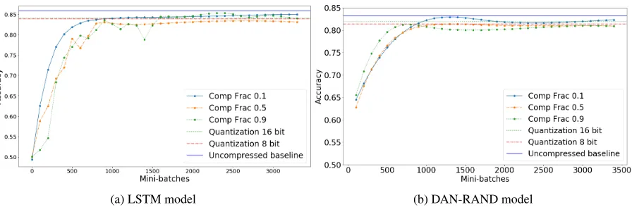
To illustrate how our proposed method benefits from re-training the model after compressing the embedding input matrix, in Fig 3 we plot the dev set accuracy for SST2 across training mini-batches for different compression percentages
Model R(%) Size(MB) Acc. Acc. Uncompressed LSTM model LSTM 0 29.34 91.78
-Quantized model (Baseline 1)
16 bit 50 17.92 90.16
-8 bit 75 10.05 89.96
-SVD: Proposed vs Offline Compression (Baseline 2) Proposed Baseline2
LSTM 10 26.76 91.71 91.07
30 21.69 91.63 90.97
50 16.62 91.54 90.87
70 10.31 91.47 90.58
90 4.89 90.94 89.83 Uncompressed DAN model DAN 0 37.03 90.18
-Quantized model (Baseline 1)
16 bit 50 25.68 89.38
-8 bit 75 16.41 88.86
-SVD: Proposed vs Offline Compression (Baseline 2) Proposed Baseline2
DAN 10 33.96 90.15 87.35
30 29.43 90.12 87.34
50 23.16 89.47 87.14
70 18.21 89.55 86.15
90 13.08 89.23 83.72
Table 3: Compression and accuracy results on the Books In-tent dataset. R(%) refers to percentage of model size reduc-tion, Size is the model size, and Acc is the classification ac-curacy. All DAN models use the DAN-RAND variant.
R and for both LSTM and DAN-RAND. For comparison, we plot the dev accuracy of 8-bit and 16-bit quantization (baseline 1) that remains stable across epochs as the quan-tized model is not retrained after compression. As a further comparison, we plot the uncompressed model accuracy on the dev which is kept stable as well (we assume this as our benchmark point). We observe that, while our compressed model starts off at a lower accuracy compared to both the un-compressed model and the quantization baseline, it rapidly improves with training and stabilizes at an accuracy that is higher than the quantization method and comparable to the original uncompressed model. This indicates that re-training after SVD compression enables us to fine-tune the layer pa-rametersWa andWbtowards the target task, and allows us
to recover most of the accuracy.
5.6
Results on Books Intent Dataset
(a) LSTM model (b) DAN-RAND model
Figure 3: Dev set accuracy vs training mini batches for various compression percentages R for the SST2 dataset
LSTM DAN-RAND
R(%) Proposed Baseline 2 Proposed Baseline 2
10 10.71 -. 1.38
-50 9.28 9.23 0.89 0.93
70 9.21 -. 0.62
-75 9.11 9.08 0.59 0.62
90 8.46 - 0.45
-Table 4: Inference Time on the SST2 test set (seconds)
plots of dev set accuracy while re-training the proposed compressed model across mini-batches and observed simi-lar trends as for SST2 (plots are omitted for brevity).
5.7
Results on Inference Time
In Table 4, for both LSTM and DAN-RAND, we report in-ference times for the SST2 test set for different compression fractions using the proposed compression vs inference times for 16-bit and 8-bit fixed point quantization (baseline 2). As expected, for our method we see a decrease in inference time as the compression fraction (R) increases. We observe sim-ilar trends for the quantization method, where 8-bit is faster than 16-bit. For similar compression rates (16-bit equivalent to 50% compression and 8-bit is equivalent to 75% compres-sion) our method and baseline 2 (fixed-point-quantization) show similar inference times. Therefore, our method does not introduce any significant latency during inference while regaining the accuracy.
6
Conclusions and Future Work
In this work, we have proposed a neural model compression method based on low rank matrix factorization that can re-duce the model memory footprint by an arbitrary proportion, that can be decided based on accuracy-memory trade-offs. Our method consists of compressing the model and then re-training it to recover accuracy while maintaining the reduced size. We have evaluated this approach on text classification tasks and showed that we can achieve up to 90% model size compression for both LSTM and DAN models, with mini-mal accuracy degradation (1%-2% relative) compared to an uncompressed model. We also showed that our methodem-pirically outperforms common model compression baselines such as fixed point quantization and offline word embedding compression for the classification problems we examined. We have also provided an analysis of our method’s effect on the model inference time and showed under which con-ditions it can achieve faster inference compared to model quantization techniques. An additional contribution of this work is the introduction of a novel learning rate scheduling algorithm, the Cyclically Annealed Learning Rate (CALR). We compared CALR to other popular adaptive learning rate algorithms and showed that it leads to better performance on the SST2 benchmark dataset. In future, we plan to evaluate the proposed compression method and the proposed CALR schedule on a larger variety of NLP tasks including sequence tagging and sequence to sequence modeling.
References
Anwar, S.; Hwang, K.; and Sung, W. 2015. Fixed point op-timization of deep convolutional neural networks for object recognition. InICASSP , 2015 IEEE International Confer-ence on, 1131–1135. IEEE.
Bengio, Y.; L´eonard, N.; and Courville, A. 2013. Estimat-ing or propagatEstimat-ing gradients through stochastic neurons for conditional computation. arXiv preprint arXiv:1308.3432. Bergstra, J., and Bengio, Y. 2012. Random search for hyper-parameter optimization. Journal of Machine Learning Re-search13(Feb):281–305.
Bojanowski, P.; Grave, E.; Joulin, A.; and Mikolov, T. 2016. Enriching word vectors with subword information. arXiv preprint arXiv:1607.04606.
Chung, J.; Gulcehre, C.; Cho, K.; and Bengio, Y. 2014. Em-pirical evaluation of gated recurrent neural networks on se-quence modeling. InNIPS 2014 Workshop on Deep Learn-ing,.
Courbariaux, M.; Bengio, Y.; and David, J. 2014. Low pre-cision arithmetic for deep learning.CoRR,abs/1412.70244.
Duchi, J.; Hazan, E.; and Singer, Y. 2011. Adaptive subgra-dient methods for online learning and stochastic optimiza-tion. Journal of Machine Learning Research12(Jul):2121– 2159.
Golub, G. H., and Reinsch, C. 1970. Singular value de-composition and least squares solutions. Numerische math-ematik14(5):403–420.
Gong, Y.; Liu, L.; Yang, M.; and Bourdev, L. 2014. Com-pressing deep convolutional networks using vector quantiza-tion.arXiv preprint arXiv:1412.6115.
Han, S.; Pool, J.; Tran, J.; and Dally, W. 2015. Learning both weights and connections for efficient neural network. InAdvances in NIPS, 1135–1143.
Han, S.; Mao, H.; and Dally, W. J. 2015. Deep com-pression: Compressing deep neural networks with pruning, trained quantization and huffman coding. arXiv preprint arXiv:1510.00149.
Hinton, G.; Vinyals, O.; and Dean, J. 2015. Distill-ing the knowledge in a neural network. arXiv preprint arXiv:1503.02531.
Hochreiter, S., and Schmidhuber, J. 1997. Long short-term memory.Neural computation9(8):1735–1780.
Hubara, I.; Courbariaux, M.; Soudry, D.; El-Yaniv, R.; and Bengio, Y. 2016. Quantized neural networks: Training neural networks with low precision weights and activations.
arXiv preprint arXiv:1609.07061.
Iyyer, M.; Manjunatha, V.; Boyd-Graber, J.; and III, H. D. 2015. Deep unordered composition rivals syntactic meth-ods for text classification. Proceedings of the 53rd Annual Meeting of the ACL.
Joulin, A.; Grave, E.; Bojanowski, P.; Douze, M.; J´egou, H.; and Mikolov, T. 2016. Fasttext. zip: Compressing text clas-sification models. arXiv preprint arXiv:1612.03651.
Keskar, N. S.; Mudigere, D.; Nocedal, J.; Smelyanskiy, M.; and Tang, P. T. P. 2016. On large-batch training for deep learning: Generalization gap and sharp minima. arXiv preprint arXiv:1609.04836.
Kim, Y. 2014. Convolutional neural networks for sentence classification. InProc. of the 2014 Conference on EMNLP.
Kingma, D. P., and Ba, J. 2014. Adam: A method for stochastic optimization.arXiv preprint arXiv:1412.6980.
Lewicki, M. S., and Sejnowski, T. J. 2000. Learning over-complete representations. Neural computation12(2):337– 365.
Lin, Z.; Courbariaux, M.; Memisevic, R.; and Bengio, Y. 2015. Neural networks with few multiplications. arXiv preprint arXiv:1510.03009.
Liu, P.; Qiu, X.; Chen, X.; Wu, S.; and Huang., X. 2015. Multi-timescale long short-term memory neural network for modelling sentences and documents. InIn Proceedings of the Conference on EMNLP 2015.
Loshchilov, I., and Hutter, F. 2016. Sgdr: Stochas-tic gradient descent with warm restarts. arXiv preprint arXiv:1608.03983.
Lu, Z.; Sindhwani, V.; and Sainath, T. N. 2016. Learning compact recurrent neural networks. InICASSP , 2016 IEEE International Conference on, 5960–5964. IEEE.
Ma, X., and Hovy, E. 2016. End-to-end sequence labeling via bi-directional lstm-cnns-crf. InProc. of the 54th Annual Meeting of the ACL 2016.
Mikolov, T.; Chen, K.; Corrado, G.; and Dean, J. 2013. Ef-ficient estimation of word representations in vector space.
arXiv preprint arXiv:1301.3781.
Pennington, J.; Socher, R.; and Manning, C. D. 2014. Glove: Global vectors for word representation. InEMNLP, 1532– 1543.
Polino, A.; Pascanu, R.; and Alistarh, D. 2018. Model com-pression via distillation and quantization. arXiv preprint arXiv: 1802.05668.
Raunak, V. 2017. Effective dimensionality reduction for word embeddings. arXiv preprint arXiv:1708.03629. Recht, B., and R´e, C. 2013. Parallel stochastic gradient algorithms for large-scale matrix completion.Mathematical Programming Computation5(2):201–226.
Sainath, T. N.; Kingsbury, B.; Sindhwani, V.; Arisoy, E.; and Ramabhadran, B. 2013. Low-rank matrix factorization for deep neural network training with high-dimensional output targets. InICASSP , 2013 IEEE International Conference on, 6655–6659. IEEE.
See, A.; Luong, M.-T.; and Manning, C. D. 2016. Com-pression of neural machine translation models via pruning.
arXiv preprint arXiv:1606.09274.
Shu, R., and Nakayama, H. 2017. Compressing word embeddings via deep compositional code learning. arXiv preprint arXiv:1711.01068.
Smith, L. N. 2017. Cyclical learning rates for training neu-ral networks. InApplications of Computer Vision (WACV), 2017 IEEE Winter Conference on, 464–472. IEEE.
Socher, R.; Perelygin, A.; Wu, J.; Chuang, J.; Manning, C. D.; Ng, A.; and Potts, C. 2013. Recursive deep mod-els for semantic compositionality over a sentiment treebank. InProceedings of the 2013 conference on empirical methods in natural language processing, 1631–1642.
Tai, K. S.; Socher, R.; and Manning, C. D. 2015. Improved semantic representations from tree-structured long short-term memory networks. arXiv preprint arXiv:1503.00075. Trefethen, L. N., and Bau III, D. 1997. Numerical linear algebra, volume 50. Siam.
Wen, W.; Wu, C.; Wang, Y.; Chen, Y.; and Li, H. 2016. Learning structured sparsity in deep neural networks. In Ad-vances in NIPS, 2074–2082.
Xue, J.; Li, J.; and Gong, Y. 2013. Restructuring of deep neural network acoustic models with singular value decom-position. InInterspeech, 2365–2369.