so.Mean minimum leMPeraNee
I l,,00 •t/BN. lit T.,
60
50
40
y
a,...n.n.DdgnoPurchased by Agricultural Research Service, 1.1.8. Department of Agriculture, for official use.
Empirical Methods of Estimating or Predicting
Evapotranspiration Using Radiation
rase d
P
REDICTIONS of evapotranspiration are basic parameters for the engi-neer or agronomist involved in plan-ning and developing water resources. Estimates of evapotranspiration are also used extensively in assessing the irriga-tion water-management efficiency of ex-isting projects, future project drainage requirements, and the magnitude of deep percolation losses under existing management practices. Water delivered to farms and fields must provide for evapotranspiration and unavoidable per-colation beyond the root zone due to unsaturated flow caused by gravity. The first is dependent on meteorological con-ditions and the vegetative characteris-tics of the crop when water is not limit-ing. The second is dependent on man-agement such as the amount of excess water applied by rainfall or irrigation, or the moisture level maintained, and it is not directly dependent on meteor-ological conditions. Actually the rela-tive amount of deep percolation be-tween irrigations under common prac-tices is more apt to be inversely rather than directly related to evapotranspira-tion. Measurement of irrigation water delivered to an area and surface runoff, coupled with reliable estimates of evap-otranspiration, provide the most practi-cal estimates of deep percolation under existing management systems. Full utilization of water resources will re-quire more reliable estimates of evapo-transpiration in the future, and these estimates must not include deep perco-lation.
Empirical methods are used for esti-mating or predicting evapotranspiration when (a) inadequate meteorological and soil-crop data are available to ap-ply complete rational equations based on the physical processes involved, (b)
the absolute accuracy of the data needed may be adequate using simple empirical equations that require much less time and effort to solve, and (c) complete rational equations often re-quire greater technical ability and ex-perience in meteorology, physics and agronomy than many users of
evapo-Paper prepared as a contribution from the
Northwest Branch, SWORD, ARS, USDA, the Idaho Agricultural Experiment Station cooperat-ing.
The author—MARVIN E. JENSEN—is research investigations leader of water management, SWORD, ARS, USDA, Snake River Conserva-tion Research Center, Kimberly, Idaho.
• Numbers in parentheses refer to the ap-pended references.
Marvin E. Jensen
MEMBER ASAE
Solar marealian (July)
BOO (ly}
Anz.•
...„,lachroola, Florida
407 7 •Madisan, Wisc.
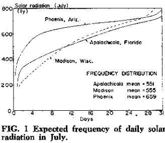
FREQUENCY OISTFSBUTION Apalachicola mean .551 Madison mean =555 Phoenixm eon •659
• Days
FIG. I Expected frequency of daily solar
radiation in July.
transpiration data have or can justify attaining.
Rationally developed empirical meth-ods of estimating or predicting evapo-transpiration, using either net or solar radiation as the primary variable, ap-proximate solutions based on the con-servation of energy or "energy balance." Energy balance has repeatedly been shown to be a reliable and conservative method of determining evapotranspira-tion for periods of time as short as one hr. Empirical methods using radiation are more reliable for both short and long-time periods than those using me-teorological parameters that are not a measure of available energy, or basic components of energy balance or mass transfer equations. However, qualified technicians have little justification in using empirical methods when the basic meteorological parameters such as net radiation, vapor pressure and tempera-ture gradients, wind speed at a pre-scribed elevation above the crop or over a standard surface, and soil heat flux are available. Preceding papers presented at this conference clearly demonstrated that reliable, rational equations are available for estimating or predicting evapotranspiration when these parameters are known.
40 50 Go 70 80
40 50 60 70 40
20 4•50 60 70
Marnray mean dew pain;
FIG. 2 Monthly mean minimum air tem-'peratures and monthly mean dew point
temperatures.
Several combination-type equations requiring three or four meteorological parameters may involve some empiri-cism and perhaps also fall in the cate-gory of this paper. However, the basic concept of the combination method was summarized in the preceding paper. Examples of methods requiring some empirical coefficients are those pro-posed by Penman in 1948, Ferguson in 1952, Budyko in 1956, and Slatyer and Mcllroy in 1961 (1, 3, 14, 19) °. Stan-hill in 1962 (20) approximated the aerodynamic component of the com-bination equation using atmometers. Energy Balance and Combination Equations
Energy balance and combination equations for the soil-crop surface are presented to clarify the notation used and as a review of basic concepts. Only the major components are shown.
LE = (1 — /1„ — A — G
[1] where (1 — OR, — R, R„, [2] thus LE = R„ — A — [3]
In these equations LE is latent heat, r is reflectance or albedo of the surface,
R,, is direct and diffuse solar radiation (short wave), A is sensible heat flux to the air (negative for heat flux from the air), G is sensible heat flux to the ground (negative for heat flux from the ground), R. t is the net long wave or thermal radiation from the ground and plant surfaces to the atmosphere, and R„ is net radiation (short and long wave). Solutions of equation [1] or [3] (rate of evapotranspiration) re-quire the determination or calculation of the components on the right side. A detailed review of energy-balance con-cepts can be found in numerous recent publications such as those by Budyko (1), Tanner (23), Tanner and Lemon (24), Jensen and Haise (10), Rijtema. (18), and Waggoner et al {28).
Combination equations generally are of the form
LE — (R„ G) + "/
+ 7 q ± 7
f d ) ti(eg e,) [4] where is the slope of the saturation vapor pressure-temperature curve,
rie dT; 7 is the psychrometric constant;
r. is the surface roughness length, d is the displacement of the zero plane of 600
200
30
Air temperature
A +
TABLE 1. SUMMARY OF A/(41 + 7 ), 7 /(A + y) AND A/y VS T
A
Computed from Smithsonian Meteorological Tables, 6th edition, 1058, equation [2], page 365, and Table 103, page 372.
A + y
30 86 0.781 0.219 3.57
35 95 0.819 0.181 4.53
40 104 0,851 0.149 5.70
deg C deg F
1 33.8 0,417 0.583
5 41 0.478 0.522
10 50 0.552 0.448
15 39 0.621 0.379
20 68 0.682 0.318
77 0.735 0.265
25
0,72 0.92 1.23 1.64 2.15 2.78
..L12r•Irilr mean (trn-nA• re.
Socrrmema. colt ..' &nage car. / ... %ors./
o.ei , 1, Vine/ 1.1 ii ,/ // ... /..
,
...P.
.4 . • r
4
I.. •
/
02 / "
/A ...I.'
0.4 0.6 C 02
FIG. 3 Monthly mean humidity as
indi-cated by difference between saturation vapor pressure at mean maximum air
perature, e,, and mean minimum air
tem-perature, e1, as compared to (e,, — e,)
where e, is the saturation vapor pressure
at monthly mean dew point temperature. e' 70 mb.
wind velocity in relation to the ground surface, u is wind speed, e, is the satu-ration vapor pressure of the air, and
ed is the actual vapor pressure of the
air. The parameters A/ (4L y) and
V (A + 7) are air-temperature weight-ing factors whose sum is 1.0. A sum-ma•y of these terms is presented in Ta-ble 1. Most combination equations as-sume that G = 0 or negligible.
EMPIRICAL RADIATION EQUATIONS
Empirical radiation equations that are rationally developed can be ex-pected to resemble equations [1] , [3], or [4]. Most would be simplified to fit one of the following forms:
LE = K, R„ [5]
LE = K, (1),, R. [6 ]
LE = K, 4 3 R A . . [7] in which K, is a crop coefficient, R, is extraterrestrial solar radiation, and 4, 0.), and 03 are net radiation, solar
radi-ation, and extraterrestrial radiation co-efficients, respectively. The products cal R1,, die B,, and 03 RA generally
rep-resent potential evapotranspiration or the upper limit of evapotranspiration that can occur from agricultural crops in either humid or arid areas sur-rounded by sufficient buffer area so that the "clothesline" effect is small or negligible. The width of the buffer strip required may be only 100 ft or less for most short, dense field crops. The crop coefficient accounts for the period of
leafarea development, minor differ -eaces between field crops when an ef-fective full crop canopy exists, (IC,
1.0), and the maturation stages of growth. Effective full-crop canopy may not mean complete ground cover, but sufficient leaf areas so as not to limit evapotranspiration.
When K, = 1.0, equations [5], [6], and [7] can be rearranged to assess the factors involved in the various co-efficients. For example, the net radia-tion and solar radiaradia-tion coefficients for daily totals represent the following terms:
LE A + G
Or — =1.0 . .
[8]
R. R„
_ LE
Oa — = 1 — r — R —
Ft, R.
A ± G R,
When considering daily totals, the value of (Ai will be approximately 1.0 when
the algebraic sum of A and G 0. The value of 4)2 at this time will be 1 r
R„ R, or about 0.75 — Re „'R, since
the reflectance is about 0.25 for most crops. A summary of observed cpi and
432 values will be presented in a later
section.
LIMITATIONS OF EMPIRICAL EQUATIONS
The major limitation of any empirical equation for estimating evapotranspira-tion is that its constants may not be ap-plicable in other climatic regimes with-out calibration. Most empirical equa-tions contain only one meteorogical pa-rameter, or at least not all of the basic parameters. Therefore, calibration does not assure the same reliability in dif-ferent climatic regimes unless the equa-tion contains the meteorological param-eters controlling or closely related to evapotranspiration. For example, in arid areas sensible heat from vast dry, unirrigated areas often contributes part of the daily heat energy for evapotran-spiration (warm air advection). This seldom occurs at significant magnitudes in humid areas. The daily rise in air temperature is a measure of the radiant energy reaching the earth's surface on a regional basis that was not utilized in evapotranspiration. Therefore, an
em-pirical equation with air temperature as the main parameter would not be as reliable for short-period estimates in humid areas as in arid areas. In con-trast, since radiant energy is the main source of heat energy in both areas, empirical equations with a radiation term can be applied with more confi-dence in either area when calibrated. The larger variability in day-to-day radiation in semihumid and humid areas, oftentimes with small changes in air temperature, is further evidence that radiation is more important than air temperature in estimating evapotran-spiration under these conditions. The expected frequency of daily solar radi-ation in July for three locradi-ations is pre-sented in Fig. 1 which illustrates that daily solar radiation is expected to devi-ate only 10 percent from the long-time mean two-thirds of the month at Phoenix, Ariz. In contrast, the expected deviation at the Florida location is ± 24 percent, and in Wisconsin ± 32 per-cent.
Eg Imm /day)
10
aspen4als AuslrOlio % . [128-3-CIT-T,.11 R.
a R.
6 C.0.6. (i / C .0.05, IT
2 4
0
A 0 2 4 6 8 10 E. (own/day)
FIG. 4 Example procedure for correcting the net radiation coefficient, cf,, using the mean air temperature—net radiation lag.
These examples illustrate that "cali-bration" of an empirical equation may be necessary to assure its accuracy when used under climatic conditions that are significantly different than those under which the equation was derived. Also, the short-period accu-racy of an empirical equation may not be the same under vastly different cli-matic conditions even though the equa-tion is "calibrated." The accuracy of an empirical equation being used in another climatic regime will depend on which meteorological parameters are used.
0.6
0,3q
Rneenix•Sr.Ir.
IA as 08 TO O 02 6A 05 0.8 1.0 3•14nthly mean I ...-e,i/e r
[9 ]
T-1 P.,•11.07 +0.3{T: TAR
Rd /NT T,. 1 get0.93+CL1IT – T„)) R.
Rn
6 8 r0
ESTIMATING METEOROLOGICAL PARAMETERS
071E.
..512V4016 . Rut 'MU OA .0.01491T-291 • ••••
r • 0.91 0.511
cola.
• 0.00891IN 7.5! v
MI •
OA 0.3! 021
80 / 50 Z-0
30 40
Meal, mcnrnly air rempsrolure
cyrtesver. N.C. • ODOM 1T-221 • • 0.99 70 80 50 60 70 EIO
(*F-40 50 60 70 40
FIG. 5 Observed increase in the ratio of
evapotranspiration from grass to solar radi-ation, 4,2, as mean air temperature
in-creases.
TABLE 2. SUMMARY OF REGRESSION EQUATIONS FOR MONTHLY MEAN VALUES OF (4, — 4, )/4' VS (e., )/e'"
Location a b Correlationcuetticient
tie. e
-r b
e' e'
c' 70 Mb
e — Several procedures for estimating
solar radiation have been satisfactorily used for many yrs. Estimates based on clear-day values and the percentage of daily sunshine are generally the most reliable (10), Solar radiation can also be reliably extrapolated between widely separated points of measurement in arid areas (9). Similarly, estimates of net radiation based on a linear relationship with solar radiation are very reliable in arid areas.
Mean dew-point temperatures also can be extrapolated between climatic stations and used with most empirical equations requiring dew points. When dew-point temperatures are not avail-able, they can be estimated using mini-mum air temperatures in humid or cool, semihumid areas (6) from which a saturation vapor-pressure value, e l , can be obtained (Fig. 2). The relationship between (ea e 1 ) and (e 2 ed ) is
essentially linear in both arid and hu-mid areas (Fig. 3). Therefore (en —
ed ) can be estimated for individual
months using a linear relationship de-rived using two points. The se two points can be obtained from mean data for January and July in the northern hemisphere which are commonly avail-able (maximum, minimum, and dew-point temperatures). If dew-dew-point data are not available, then saturation vapor pressure at minimum temperatures could be used with en as an index of humidity. This index would underesti-mate (e2 — ed ) by as much as 25
per-cent in arid areas as shown in Fig. A summary of (en — e 1 ) vs (e2 ed ) for additional locations is presented in Table 2. The excellent correlation is due to the use of e., in both variables, and since the saturation vapor pres-sure-temperature relationship is non-linear, differences between minimum temperature and dew-point tempera-ture have small effects.
NET RADIATION COEFFICIENTS
Numerous studies have shown that net radiation accounts for most of the variability in evapotranspiration when soil water and vegetative cover are not
limiting. The minimum value of cp, will be about 4,/(6. + 7 ) (19). Gen-erally 4 will be near 1.0 in semihu-mid to husemihu-mid areas with a small "loop" effect occurring during the season be-cause of the lag in sensible heat in the air and soil. Simple linear-regression equations derived from observed data for a given area such as those presented by Tanner (23) and Pruitt (15) can be used to estimate evapotranspiration. Pruitt presented two regression equa-tions — one for the period of increasing sensible-heat storage in the air and soil and the other for the period of decreas-ing sensible heat. In areas where ad-vection is severe, short-period values of yth often exceed 1.0 and may reach 1.8 as illustrated by the data of Frits-•chen (4), Mcllroy and Angus (12), Pruitt (15), and van Bavel (27). Thus 0, cannot be assumed constant in a given area, nor can it be assumed to be, near 1.0 for all areas for estimating pur-poses. If complete meteorological data are available, then one of the combina-tion equacombina-tions (with calibracombina-tion) could be used to obtain good estimates of potential evapotranspiration when net radiation is known. Other procedures must be used when supporting meteor-ological data are inadequate, or the basic meteorological data also must be estimated.
The energy balance components af-fecting the magnitude of 0, in equa-tion [5] are A and G. During the pe-riod when soil and air temperatures are increasing, part of the daily net radiation on a regional basis is con-verted to sensible heat in the air and soil. The opposite occurs when air and soil temperatures are decreasing. There-fore, one would expect a "loop" effect in the value of 4) , on a regional basis due to the thermal lag of the soil and air mass. This loop effect could be re-lated to 1.0 — C(dT Mt) 'RI, in humid areas where T is mean daily air tem-perature, t is time, and C is a. coefficient representing a "specific heat capacity" for the air and soil as related to the mean rate of air-temperature change measured at shelter height. In irrigated areas, or areas where warm-air advec-tion ma y significantly affect 0,, the above relationship would probably
re-Bismarck, N.D. 0.008
Yakima. Wash. 0:011
Brownsville, 'rex. 0.023
Sacramento, Calif. 0.015
Fresno, Calif. 0.032
Dodge City, Kans. 0.022
Yuma, Ariz. 0,020
Phoenix, Ariz.Grand Junction, Colo, 0,0180,047
quire separate coefficients for the pe-riods when regional sensible heat is in-creasing and when regional sensible heat is decreasing. However, under these conditions C may not be constant and the entire equation would become more complex. If an empirically de-rived relationship is to be used, it must be an extremely simple relationship to justify its use over more rational equa-tions. One such relationship is as fol-lows:
LE
= 1 — T—T ro 4,4
fi
n [10] R„
where T is mean air temperature, T,„ is mean air temperature for a given value of at a given location if no "loop effect" exists. Therefore, Trn can be obtained from a linear relationship between mean air temperature and net radiation in January and July when
dT /dt 0. 4 is a dimensionless local calibration constant or a variable that may be related to some other climatic parameters such as vapor-pressure def-icit and wind speed. When 4)4 is
con-sidered a constant, its magnitude can be evaluated when dT/dt 0 which normally occurs in January and the lat-ter part of July in the northern hemis-phere. Equation [10] was evaluated using grass evapotranspiration data from Mcllroy and Angus (12) and Pruitt (18) (Fig. 4). The weighted mean value of 44 for Aspendale, Aus-tralia was 0.29. Combining the con-stants results in a simple "calibrated" prediction equation for potential evapo-transpiration from grass using net radia-tion and air temperature as shown in Fig. 4. These modifications essentially removed the loop effect shown by Mc-Bray and Angus when using the mean value of 0, = 1.2.
A similar analysis was made using mean grass data from California (16). In this case (/), was —0.07 when T was increasing or T < Tr. and 0.04 when T > T,,,. Substitution in equation [10] resulted in the equations shown in Fig. 4. These equations removed most of the loop effect present using the mean value of 0 2 0.98.
An evaluation of these equations for estimating evapotranspiration for
indi-0.948 0.998
0.906 0,998
0.874 0.997
0.892 0,998
0.824 0.998
0.774 0,998
0.729 0.998
0.706 0.997
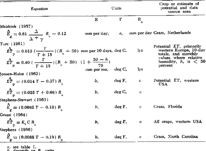
Makkink ( 1937 )
P. 0.81 A R --0.12 mm per day,
g A + 7
A =
0.013 ( T ) ( R .+. 30) min per 10 days. deg C,1, T + 15
A . 0,40 ( T )(R -i- 50) ti T -4- 15
Jensen-Haise ( 1963 )
El'
u=
(0.014 T — 0.37 ) R b. deg F,
A- --- (0.025 T + 0.08) R b,
P s
Stephens-Stewart ( 1963)
A
R = ( 0.0082 7' -- 0.19) R 3, deg F,
g s
Grassi (1964 )
A
il . Ki C R ll b, deg F, Stephens (1966)
Pg .
( 0.0088 T --0.19) Rs 3, deg F.Ttire (1981)
deg C,
• Potential ET, western USA
Grass, Florida
• AR crops, western USA
• Grass, North Carolina (1 + 50 — h
70
inm per ma, deg C, lys
a, see table 1.
3, depends on 11 units.
c, equivalent depth of evaporation, i.e., min per day, in. per day, etc.
rein per day Grass, Netherlands
Potential ET, primarily western Europe, 10-day totals, and monthly values where relative humidity, h, is < 50
percent
lys
vidual months resulted in a standard error of 0.5 mm per day for both Aspendale and Davis. The standard er-ror using 4 = 1.2 for Aspendale was 0.62 mm per day, and when using (A t
= 0.98, the standard error was 0.75 mm per day for Davis. The tempera-ture lag adjustment improves the esti-mates.However, if sufficient data are available to estimate R„, one can sel-dom justify using this approach over one of the combination equations since very little additional data are needed.
SOLAR RADIATION COEFFICIENTS
The value of 02, as shown in equa-tion [9], will be about 0.75 — Ret/115 in July and January in humid areas at which time (mean daily) A + G 0. Since
R
et;'R
5 generally decreases with increasing solar radiation, an increase in rp.i is expected as R„ increases. This increase can be predicted by estimat-ingR
E. t . An adjustment for the lag in sensible heat in the air and soil could also he incorporated as was done for 4)1 . In addition, another adjustment must be made in areas where warm-air advection may occur since A + Gfor individual irrigated fields in July. If all of these adjustments had to he made independently, the resulting em-pirical equation would be cumber-some to use, and large errors may re-sult when inexperienced personnel used this procedure. Instead, since the air temperature vs solar radiation lag re-flects the lag in sensible heat stored in the soil and air, air temperature gen-erally increases on a regional basis with increasing R, and since the magnitude of advection is partially related to air temperature, one would expect a
gen-era) increase in 422 as mean air temper-ature increases. This increase was ap-parent in evapotranspiration data ob-tained throughout western USA, Jen-sen and liaise (10). Mean monthly lysimeter data from Aspendale, Aus-tralia, Mcllroy and Angus (12); Davis, Calif., Pruitt (16); Waynesville, North Carolina, [Fry et al (5) and Gilbert and van Ravel (7) as summarized by Stephens (21) ], are presented in Fig. 5 to illustrate the linear relationship of vs mean air temperature. The mag-nitude of Eg ., R, is greater under more arid conditions as is the slope of the regression equations. Mean air-temper-ature data reported for Aspendale by Mcllroy and Angus is the mean of 09:00 and 15:00 hour observations. The normal mean air temperature computed from the maximum and minimum would be lower and the slope of the regres-sion equation in Fig. 5 would be even greater. The Aspendale site is adjacent to Port Phillip Bay which would in-fluence the air temperature-radiation relationship, and the lysimeters were irrigated up to four times per day which may have resulted in unusually high evapotranspiration rates for grass. A similar regression equation was ob-tained at Davis using mean air tempera-ture at the Sacramento, Calif., airport. However, since the air temperature is higher at the airport, the coefficient was 0.0091 instead of 0.0099. The in-tercept of the x axis was about the same (17 F) and the correlation coefficient was 0.97. Therefore, it is not essential that air temperature be measured over the field, however, the coefficients may he slightly different.
Several regression equations for
esti-Crop or estimate of
Potential and data source area
L£ /R,
(11 Jensen-maiss (19631 121 Grass -Calif. (Pruitt)
at Grass -N.Corolina 141 Grass -Florida (51 Makkink 11957)
Alfalfa-Arizona
(won BOV81,1966) •
(4)
0.2
-5 0 2q 30 40
12q 40 60 50 100 Mean Air Temperature 1 •F1
FIG. 6 Empirical regression equations re-lating the solar radiation coefficient, 0 2 , to mean air temperature, and observed sin-gle day values for alfalfa in Arizona. mating evapotranspiration and some single-day values are presented in Fig. 6 to illustrate the differences due to climate and crops. The length of the lines represent the range of data used or variations in air temperature in the area where the data were obtained. The equation by Makkink (11) is about as good as Penman's equation for 10-day means in the Netherlands (17). The three equations for grass reflect primarily climatic differences. The re-gression equation by Jensen and Haise (10) represents data from crops other than grass and may reflect the influ-ence of the roughness and leaf area of the crop. The alfalfa data from van Ravel (27) are single-day values in Arizona. The two high points repre-sent severe advective conditions. These and several other estimating equations are summarized in Table 3. There are other estimating procedures that in-volve solar radiation such as those presented by Olivier (13) and Thomp-son (25). Turc's (26) equation gen-erally will fall in the same area as the others in Fig. 6, except that the curve tends to flatten as T increases. The gen-eral humidity of a region and de-gree of warm-air advection appear to be the major climatic factors influencing variation in the slope of the lines in Fig. 6. The coefficient C in Grassi's (8) equation is a product of several di-mensionless coefficients representing such parameters as air temperature, crop stage of growth, cloud cover, etc. A detailed summary of more recent de-velopments in using this general equa-tion for estimating evaporaequa-tion from water surfaces is presented by Chris-tiansen (2).
The major advantages of empirical equations using solar radiation are sim-plicity, "calibration" for an area is not .difficult, and estimates have sufficient reliability for most engineering or wa-ter-management applications. Solar ra-diation is measured at a large number of locations throughout the world. Mean values can be estimated for most areas using clear-day or extraterrestrial
val-TABLE 3. SUMMARY OF SOME EMPIRICAL SOLAR RADIATION EQUATIONS
Equation Units
12
1.0
0.8
Ry.proms, COI'. I
(1-yminnor - P.M).
•
.1. • 0.00991T-I R, n
1961
0,1FMAIAJJA5 0NDJ FMANIJJASON
FIG. 7 A comparison of estimated
evapo-transpiration from grass using a calibrated empirical solar radiation-mean air tem-perature equation with measured evapo-transpiration.
ues and percent of sunshine or cloud cover (10). Also interpolation between locations separated by several hundred miles usually provides adequate esti-mates except where orographic features may create localized cloud cover varia-tions (9). The second major advantage is that solar radiation equations, prop-erly calibrated, give estimates that are in phase with measured values as illus-trated in Fig. 7 using mean monthly data.
A summary of the standard error for daily, mean 5-day, mean 10-day, and mean monthly estimates using only T
and R, for Davis, California, is pre-sented in Table 4. The standard error during the summer months ranges from about 0.015 in. per day for monthly means to 0.035 for daily values. The coefficient of variability for these months ranges from 8 to 15 percent. The standard error increases during the fall months largely because of windy, high advection days. Since wind is not a variable in the estimating equation used, only that portion of adverted en-ergy related to mean air temperature is considered. Wind speed could easily be incorporated in an estimating equa-tion for arid areas when standard wind speed data are available. Solar radia-tions equaradia-tions are also reliable in hu-mid areas. Stephens and Stewart (22) found that a solar radiation equation gave more reliable estimates in humid areas of Florida than temperature methods.
One problem associated with a solar radiation - air temperature relationship is the determination of the slope of the regression line, or the mean tempera-ture coefficient, and the intercept of the temperature axis. T, for new areas. There are three possible procedures for doing this: (a) calibrate the equation using accurately measured ET data col-lected throughout the season from an area having similar climatic conditions; (b) calibrate using January and July data, or use July data in the northern hemisphere and data near the beginning and end of the growing season, and Cc) relate the temperature coefficient and temperature intercept to one or more
climatic factors that are related to hu-midity.
An example of the last procedure for estimating 432 , when very limited data are available, is as follows:
4132 = GT O' - T.) [11]
where CT is a temperature coefficient normally determined as a constant for a given area. Preliminary data indicate that CT can be estimated if only air-temperature data are available using the following expression and tempera-ture data during the month of maxi-mum mean air temperature. In tropi-cal areas having dry and rainy periods, coefficients should be derived for each period.
CT
-where
1
[12]
Cl + C2 CH
C A 37.5 mmHg
e, e, e, - e t
[13]
The value of 50 mb or 37.5 mm Hg. is about the maximum value found any-where for (e• - e 1 ). Thus the smallest value of CH 1. (C2 13 F or 7.3 C depending on the scale used.)
The intercept of the temperature axis, T„ increases as the slope of the line increases and as humidity increases.
T. can he estimated using the
follow-ing equation derived from data in the western United States, North Carolina, and Florida (C H < 2.8).
T. = -9 + 1.8 C2,/ + 2400 CT [14] for use with mean air temperature in deg F and
T.= -23 + C2H ± 750 CT , [15] for use with mean air temperature in deg C. Thus an estimate of potential evapotranspiration can be obtained us-ing the followus-ing equations with mean air temperature in deg F or C.
A T
ET ---R, (T in deg F)
48 + 13 CH
[181
ET T (T in deg C)
27 + 7.3 CH
[17]
1.2 Ke 1.0
0.8 OS
0.4
02
000 20 40 60 80 100
Planting to Heading .(%} 0 20 40 60 Days after Heading
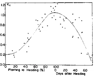
FIG. 8 An example of a crop coefficient curve relating evapotranspiration at vari-ous growth stages of grain sorghum to esti-mated potential evapotranspiration.
Equations [16] and [17] should be used only when mean
is above 50 F or 10 C. air temperatureBelow this tern-perature the estimates for short grass should be used.
Estimates for well-watered short grass can be obtained by using C, 85 F or 47 C.
When estimates or predictions of evapotranspiration are needed for vari-ous stages of crop development, then potential evapotranspiration obtained using equations [16] or [17], or a combination equation, can be multiplied by a crop coefficient K.
ET = K, ETt, . [18]
A typical example of the variation ex-pected in a crop coefficient is indicated in Fig. 8. The data points represent observed evapotranspiration values. The magnitude near planting will be influ-enced by the frequency of rainfall that may keep the soil surface moist for longer periods of the time. The curve for grain sorghum was obtained in semi-arid to semi-arid areas where the soil sur-face dries rapidly after an irrigation. Similar curves for about 15 different crops will be available within a yr from the author.
SUMMARY AND CONCLUSIONS
An analysis of empirical equations for estimating or predicting evapotran-spiration using radiation is presented. Factors affecting the use, reliability and application of these equations to new areas are discussed. Estimates of
me-1962
50 mb
TABLE 4. SUMMARY OF STANDARD ERROR OF EVAPOTRANSPIRATION ESTIMATES FOR GRASS AT DAVIS, CALIF., JULY 1939 TO JUNE 1963
( Data courtesy oW. 0. Pruitt)
Month ( in. per day )Mean Standard error (io. per day )
Daily 5-daymeans 10-daymeans Monthlymean
January
February 0.0290.073 0.0150.024 0.0090.018 ) 0.006 .1 0.008 March
April 0.0920.149 0.0240.023 0.0130.015 0.012 l 0.032
May
June 0.1920,269 0.0300.039 0.0180.028 0.019 3. 0.010
uly
August 0.2730.220 0.0250.033 0.0170,029 ) 0.021 0.021
September
October 0.1780.117 0.0260.033 0.0320,026 0.02.5 0.030
November
teorological parameters or extrapolation between widely separated points of measurements enable more rational em-pirical equations to be used even when climatic data are not readily available. Empirical equations using radiation as the primary variable provide ade-quate and reliable estimates of evapo-transpiration for most engineering pur-poses when limited meteorological data are available. Their use does not re-quire much skill, and the time and ef-fort required are minimal. The esti-mates or predictions approximate the energy balance equation. Empirical methods using radiation generally pro-vide more reliable estimates than those based on air temperature as the pri-mary variable, and are simple to use. References
1 Budyko, M. I. The heat balance of the earth's surface. (Teplovoi baler's zemnoi pover-khnosti. Gidrometeorologischeskoe izdatel'stvo, Leningrad, 225 pp., 1958) Translated by Nina A. Stepanova, Office of Climatology, U.S. De. of Commerce, Weather Bur. PB 131092, Wash-ington, D.C., 1958.
2 Christiansen, J. E. Estimating pan evapora-tion and evapotranspiraevapora-tion from climatic data. ASCE, Methods for Estimating Evapotranspira-tion ling. and Drain. Specialty Conf. 193-234, 1986.
3 Ferguson, J. The rate of evaporation from
shallow ponds. Austr. J. Sci. Res. A 5:315430, 1952.
4 Fritschen, Leo J. Evapotranspiration rates of field crops determined by the Bowen ratio method. Agron. Jour. 58:339-342, 1968.
5 Fry, A. S., at al. Annual reports of coopera-tive research projects in western North Carolina. TVA and North Carolina State College. Agr. and Eng., 1958-58.
6 Gentilli, J. Estimating dew point from minimum temperature. Bul. Amer. Meteorol. Soc. 36:0)128-131, 1955.
7 Gilbert, M. J. and van Bavel, C. H. M. A simple field installation for measuring maximum evapotranspiration. Trans. Amer. Geoph. U. 36:(8) 937-942, 1984.
8 Grassi, Carlos Julian. Estimation of evapo-transpiration from climatic formulas. M.S. thesis, Coll. of Eng., Utah State Univ., Logan. 101 pp., 1964.
9 Jensen, M. E. Discussion: Irrigation water requirements of lawns. 3. brig. and Drain. Div., Amer. Soc. Civil Eng. Proc. 92:(IR1)95-100, 1966.
10 Jensen, M. E., and liaise, H. R. Estimat-ing evapotranspiration from solar radiation. J. Irrig. and Drain. Div., Amer. Soc. Civil Eng. Proc. 89:(1R4)15-41, 1963.
11 Makkink, G. F. Testing the Penman for-mule by means of lysimeters. Jour. Inst. Water Eng. London 11:277-288, 1957.
12 Mellroy, I. C., and Angus. D. E. Grass, water and soil evaporation at Aspendale. Agr, Meteorol, 1:201-224, 1984.
13 Olivier, Henry. Irrigation and Climate. Edward Arnold, Ltd. (Publishers), London, 250 pp., 1961.
14 Penman, IL L. Natural evaporation from open water, bare soil, and grass. Proc. Roy. Soc. London (A) 193:120-145, 1948.
15 Pruitt, W. 0. Cyclic relations between evapotranspiration and radiation. Transactions of the ASAE 7:(3)271-275, 280, 1984.
16 Pruitt, W. O. Unpublished data received through personal communication. December 1966.
17 Rijtema, P. E. Calculation methods of potential evapotranspiration. Tech. Bul. 7, In-stitute for Land and Water Mgt. Res., Wagen-ingen, The Netherlands. 10 pp., 1959,
18 Rijtema, P. E. An analysis of actual evap-otranspiration. Agr. Res. P.pts. No. 659, In-stitute for Land and Water Mgt, Res., Wagen-ingen, The Netherlands, 107 pp., 1965.
19 Slatyer, R. 0., and Mellrmi, I, C. Practi-cal rnicroclimatology. CSIRO, Melbourne. 310 pp., 1961.
20 Staribill, G. The use of the Fiche evap-orimeter in the calculation of evaporation. Qtriy. Jour. Roy. Meteorol. Soc. 88:80-82, 1962.
21 Stephens, 3. C. Discussion: Estimating evaporation from insolation, J. Hydr. Div., Amer. Soc. Civil Eng. Proc. 91:(HT5)171-182, 1965.
22 Stephens, J. C., and Stewart, E. H. A comparison of procedures for computing evapora-tion and evapotranspiraevapora-tion, Pub. No. 62, Inter-natl. Assn. of Sci. Hydra, Interne& Union of Geod. and Geoph, 123-133, 1963.
23 Tanner, C. B. Energy balance approach to evapotranspiration from crops. Soil. Set Soc. Amer. Proc. 24:1-9, 1960.
24 Tanner, C. B., and Lemon, E. R. Radiant energy utilized in evapotranspiration. Agron. Jour. 54:207-212, 1962.
25 Thompson, C. B. Irrigation water require-ments in Texas. J. brig. and Drain. Div., Amer. Soc. Civil Eng. Proc. 90:(1R3)17-40, 1964.
26 Turc, L. Evaluation des besoins en eau d'irrigation, evapotranspiration potentielle, for-mula climatique simpiifiee at mice a jour (In French) (English title: Estimation of irrigation-water requirements, potential evapon.anspiration: a simple climatic formula evolved up to date.) Ann. Agron. 12:13-49, 1961.
27 van Bevel, C. H. M. Potential evapora-tion: the combination concept and its experi-mental verification. Water Resources Res. 2:(3) 455-467, 1966.