Multiobjective Optimization

(1)

Multiobjective Optimization — New Formulation

and Application to Radar Signal Processing

A THESIS SUBMITTED IN PARTIAL FULFILLMENT OF THE REQUIREMENTS FOR THE DEGREE OF

Master of Technology

in

Telematics and Signal Processing

By

VIKAS BAGHEL

Roll No: 207EC105

Department of Electronics and Communication

National Institute of Technology

(2)

Multiobjective Optimization — New Formulation

and Application to Radar Signal Processing

A THESIS SUBMITTED IN PARTIAL FULFILLMENT OF THE REQUIREMENTS FOR THE DEGREE OF

Master of Technology

in

Telematics and Signal Processing

By

VIKAS BAGHEL

Roll No: 207EC105

Under the Supervision of

Prof. Ganapati Panda

FNAE, FNASc.

Department of Electronics and Communication

National Institute of Technology

Rourkela, India

2009

(3)

National Institute of Technology

Rourkela

CERTIFICATE

This is to certify that the thesis entitled, “Multiobjective Optimization — New

Formulation and Application to Radar Signal Processing ”submitted byVikas Baghel

in partial fulfillment of the requirements for the award of Master of Technology Degree in

Elec-tronics & Communication Engineering with specialization in Telematics and Signal

Processingduring 2008-2009 at the National Institute of Technology, Rourkela (Deemed Uni-versity) is an authentic work carried out by him under my supervision and guidance.

To the best of my knowledge, the matter embodied in the thesis has not been submitted to any other University / Institute for the award of any Degree or Diploma.

Date Prof. G. Panda (FNAE, FNASc)

Dept. of Electronics & Communication Engg. National Institute of Technology Rourkela-769008 Orissa, India

(4)

Acknowledgment

First and foremost I offer my sincerest gratitude to my supervisor, Prof. Ganapati Panda, who is supported me throughout my project with patience and knowledge whilst allowing me the room to work in my own way. Besides our weekly meetings, he was always willing to answer my questions and to help me to overcome my doubts. I feel proud that I am able to finish his toughest classes successfully. He always pushed me to my limits to get the best out of me. I attribute the level of my Masters degree to his encouragement and efforts and without him this thesis, too, would not have been written or completed. One simply can not wish for a better or friendlier supervisor.

Sincere thanks to Prof. S. K. Patra, Prof. K. K. Mahapatra, Prof. G. S. Rath, Prof. S. Meher , Prof. S.K.Behera, Prof. Punam Singh and Prof. Ajit Kumar Sahoo for their constant cooperation and encouragement through out the course.

I am privileged to express my sincere gratitude to Prof. K. Rajarajeswari for their inspiration and co-operation in collecting secondary information. I gratefully acknowledge Mr. P. Srihari for his advice, supervision, and crucial contribution, which made him a backbone of this research and so to this thesis.

I also extend my thanks to entire faculty of Department of Electronics and Com-munication Engineering, National Institute of Technology Rourkela, Rourkela who have encouraged me throughout the course of Masters Degree.

I would like to thank my friends, especially Satyasai Jagannath Nanda, Pyari Mo-han PradMo-han, Nithin V george, Pavan kumar Gorpuni, S.K.Verma and Jyoti for their help during the course of this work. I am also thankful to all my classmates for all the thoughtful and mind stimulating discussions we had, which prompted us to think beyond the obvious.

And finally thanks to my parents and my sisters, whose faith, patience and teaching had always inspired me to walk upright in my life. Without all these beautiful people my world would have been an empty place.

Vikas Baghel

(5)

The present thesis aims to make an in-depth study of Multiobjective optimization (MOO), Multiobjective algorithms and Radar Pulse Compression. Following the approach of bacteria foraging technique, a new MOO algorithm Multiobjective Bacteria Foraging Optimization (MOBFO) has been proposed in this thesis. We compared the performance of our proposed algorithm with existing algorithms Nondominated Sorting Genetic Algo-rithm (NSGA-II) and Multiobjective Particle Swarm Optimization (MOPSO) for differ-ent test functions. In radar signal processing Pulse Compression is used for high range resolution and long range detection. The classical methods for Pulse Compression of the received signal use matched filter and mismatched filter. For improving the perfor-mance of pulse compression, a new problem formulation has been constructed that uses constrained function optimization with the help of Particle Swarm Optimization (PSO). Artificial Neural Network (ANN) is being used for Pulse Compression that achieves a sig-nificant supression of the sidelobes. Functional Link Artificial Neural Network (FLANN) has been proposed for better sidelobes reduction than Multi Layer Perceptron (MLP) network with both lower computational and lower structural complexity. MOO approach has been proposed to use with Radial Basis Function (RBF) for Pulse Compression that improves the accuracy and complexity of RBF network.

(9)

LIST OF FIGURES

2.1 An example of a MOP with two objective functions: Cost and Efficiency . 11

2.2 MOP Evaluation Mapping . . . 11

3.1 Crowding-distance Calculation . . . 16

3.2 NSGA Procedure . . . 17

3.3 MOPSO Flow Chart . . . 19

3.4 Archive Controller . . . 21

3.5 Adaptive Grid . . . 22

3.6 MOBFO Flow-chart . . . 25

4.1 Nondominated Pareto Front . . . 30

4.2 Nondominated Pareto Front for SCH problem . . . 34

4.3 Nondominated Pareto Front for KUR problem . . . 36

4.4 Nondominated Pareto Front for DEB1 problem . . . 37

4.5 Nondominated Pareto Front for DEB2 problem . . . 39

5.1 Pulse Compressed Signal . . . 44

5.2 FLANN Structure . . . 51

5.3 FLANN : Mean Square Error Plot . . . 53

5.4 FLANN : Peak Signal to Side-lobe Ratio (SSR) for the 13 element barker code . . . 54

5.5 FLANN : Noise performance for the 13 element barker code for 3 dB SNR 56 5.6 FLANN : Compressed waveforms of overlapped 13 element barker code with 7 delay apart . . . 57

5.7 FLANN : Correlated output for Doppler Shift . . . 58

(10)

6.1 Radial Basis Functions (RBF) Network . . . 64 6.2 Chromosome - Center representation . . . 65 6.3 PRBF : Pareto Fronts . . . 67 6.4 PRBF : Noise performance for the 13 element barker code for 5 dB SNR . 69 6.5 Input waveform on additional of two 4-delay-apart 13-element Barker

se-quence having same amplitude . . . 71 6.6 PRBF : Compressed waveforms of overlapped 13 element barker code with

15 delay apart . . . 72 6.7 PRBF : Doppler Shift Performance for 13 element barker code . . . 73

(11)

LIST OF TABLES

4.1 Computational Time (in sec) required by each Algorithm for the SCH Test

Function . . . 33

4.2 Results of the Convergence Metric for the SCH Test Function . . . 34

4.3 Results of the Diversity Metric for the SCH Test Function . . . 35

4.4 Computational Time (in sec) required by each Algorithm for the KUR Test Function . . . 35

4.5 Results of the Convergence Metric for the KUR Test Function . . . 35

4.6 Results of the Diversity Metric for the KUR Test Function . . . 35

4.7 Computational Time (in sec) required by each Algorithm for the DEB-1 Test Function . . . 37

4.8 Results of the Convergence Metric for the DEB-1 Test Function . . . 38

4.9 Results of the Diversity Metric for the DEB-1 Test Function . . . 38

4.10 Computational Time (in sec) required by each Algorithm for the DEB-2 Test Function . . . 38

4.11 Results of the Convergence Metric for the DEB-2 Test Function . . . 39

4.12 Results of the Diversity Metric for the DEB-2 Test Function . . . 40

5.1 PSO : Comparison of SSR (in dB) . . . 49

5.2 PSO : Comparison of SSR (in dB) for 13 element Barker code for different noisy condition . . . 49

5.3 PSO : Comparison of SSR (in dB) for 35 element Combined Barker code for different noisy condition . . . 50

5.4 FLANN : Comparison of SSR (in dB) . . . 55

5.5 FLANN : Comparison of SSR (in dB) for 13 element Barker code for dif-ferent noisy condition . . . 55

(12)

5.6 FLANN : Comparison of SSR (in dB) for 21 element Optimal code for

different noisy condition . . . 55

5.7 FLANN : Comparison of SSR (in dB) for 35 element Combined Barker code for different noisy condition . . . 55

5.8 FLANN : Comparison of SSR (in dB) for 13 element Barker code for Range Resolution of two targets . . . 58

5.9 FLANN : Comparison of SSR (in dB) for Doppler shift . . . 59

6.1 Parameter Setting for BNSGA . . . 66

6.2 PRBF : Comparison of SSR (in dB) . . . 68

6.3 PRBF : Comparison of SSR (in dB) for 13 element Barker code for different noisy condition . . . 68

6.4 PRBF : Comparison of SSR (in dB) for 21 element Optimal code for dif-ferent noisy condition . . . 68

6.5 PRBF : Comparison of SSR (in dB) for 35 element Combined Barker code for different noisy condition . . . 70

6.6 PRBF : Comparison of SSR (in dB) for 13 element Barker code for Range Resolution of two targets . . . 70

6.7 PRBF : Comparison of SSR (in dB) for 35 element Combined Barker code for Range Resolution of two targets . . . 70

6.8 PRBF : Comparison of SSR (in dB) for Doppler shift . . . 74

(13)

Chapter 1

Introduction

Background Motivation Present Work Thesis Organization

(14)

CHAPTER 1 INTRODUCTION

1.1 Background

Most real-world search and optimization problems are naturally posed as multiobjective optimization problem (MOP). The majority of engineering optimization is the MOP, sometimes it need to make multiple targets all reach the optimal in a given region, but it is regrettable that goals are generally conflicting. A MOP differs from a single-objective optimization problem because it contains several objectives that require optimization. When optimizing a single objective problem, the best single design solution is the goal. But for MOP, with several (possibly conflicting) objectives, there is usually no single optimal solution. Therefore, the decision maker is required to select a solution from a finite set by making compromises. A suitable solution should provide for acceptable performance over all objectives.

Many fields continue to address complex real-world MOPs using search techniques developed within computer engineering, computer science, decision sciences, and opera-tions research. The potential of evolutionary algorithms for solving MOPs was hinted as early as the late 1960s by Rosenberg [1.1]. However, the first actual implementation of a multiobjective evolutionary algorithm (MOEA) was produced until the mid-1980s by David Schaffer in his doctoral dissertation [1.2]. Since then, a considerable amount of re-search has been done in this area, now known as evolutionary multiobjective optimization (EMOO).

To improve the performance in pulse radar detection, pulse compression technique [1.3], which involves the transmission of a long duration wide bandwidth signal code, and the compression of this received signal to a narrow pulse, is always employed. In practice

(15)

CHAPTER 1. INTRODUCTION

two different approaches are used to obtain pulse compression. The first one is to use a matched filter; here codes with small sidelobes in their autocorrelation function (ACF) are used [1.3, 1.4]. The second approach to pulse compression is to use inverse filters of two kinds, namely, non-recursive time invariant causal filter [1.5] and recursive time variant filter [1.6]. Two different approaches using a multi-layered neural network, which yield better signal-to-sidelobe ratio (SSR) (the ratio of peak signal to maximum sidelobe) than the traditional approaches have been reported in [1.7-1.9]. In the first, a multi-layered neural network approach using back-propagation (BP) as the learning algorithm is used [1.7, 1.10]. Whereas in the second approach, Radial Basis Function (RBF) network approach, using supervised selection of centers learning strategies, has been used [1.11].

1.2 Motivation

The main motivation for using MOEAs to solve MOPs is because MOEAs deal simul-taneously with a set of possible solutions (the so-called population) which allows us to find several members of the Pareto optimal set in a single run of the algorithm, instead of having to perform a series of separate runs as in the case of the traditional mathemat-ical programming techniques [1.12, 1.13]. The Pareto-optimal front can be exploited to select solutions appropriate for each particular application without having to weight the objectives in advance or reduce the multiple objectives in some other way. Additionally, MOEAs are less susceptible to the shape or continuity of the Pareto front ( e.g. , they can easily deal with discontinuous and concave Pareto fronts), whereas these two issues are known problems with mathematical programming.

Artificial Neural Networks (ANNs) are computational tools inspired by biological ner-vous system with applications in science and engineering[1.14 - 1.17]. This work is about a kind of ANN for applications in multivariate nonlinear regression, classification and times-series called Radial Basis Function (RBF) Network [1.14, 1.18]. Although ANNs have usually achieved good performances in several domains, those performances and the ANN training process are directly influenced by an appropriate choice of the network ar-chitecture. Unfortunately, the space of network architectures is infinite and complicated and there is no general purpose, reliable, and automatic method to search that large space. When the Trial and Error method [1.19, 1.20] is employed, different values for the network parameters must be selected, trained and compared before the choice of an ultimate network. The disadvantage of this method becomes more apparent if, after the choice of the best values, the patterns set is changed, making necessary to restart the design process. This search can be done more efficient if heuristics are used to guide it. Multiobjective optimization approach is one of the standard techniques of searching in

(16)

complicated search spaces [1.21]. So one of the reasons to apply MOGAs to the RBF Net-works is due to the complex nature of their optimization which involves aspects of both numerical and combinatorial optimization with two objective functions, one for accuracy and other for complexity of network [1.22].

1.3 Present Work

This thesis is organized in such a way that its contents provides a general overview of the field now called evolutionary multiobjective optimization (EMO), which refers to the use of evolutionary algorithms to solve multiobjective optimization problems. We have proposed a new MOO algorithm Multi Objective Bacteria Foraging Optimization (MOBFO), following the approach of bacteria foraging technique. We have compared the performance of our proposed algorithm with existing algorithms NSGA-II and MOPSO for different test functions. For improving the performance of pulse compression in Radar detection, we have constructed a new problem formulation that uses constrained function optimization with the help of Particle Swarm Optimization (PSO). Traditionally, Artificial Neural Network (ANN) is being used for Pulse Compression that achieves a significant suppression of the sidelobes. Functional Link Artificial Neural Network (FLANN) has been proposed by us for better sidelobes reduction than Multi Layer Perceptron (MLP) network with both lower computational and lower structural complexity. We have also proposed the use of MOO approach to use with Radial Basis Function (RBF) for Pulse Compression that improves the accuracy and structure complexity of RBF.

1.4 Thesis Organization

Chapter-1 Introduction

Chapter-2 Multiobjective Optimization

Most multi-objective optimization methods use the concept of domination in their search. Thus, in this chapter, we have presented definitions for domination, a non-dominated set and a Pareto-optimal set of solutions.

Chapter-3 Multiobjective Evolutionary Algorithms

In this chapter, we have reviewed two most popular multiobjective optimization algo-rithms, NSGA-II and MOPSO. Here, we also proposed a new multiobjective algorithms based on the bacteria foraging technique, named Multiobjective Bacteria Foraging Opti-mization (MOBFO).

(17)

Chapter-4 Performance Evaluation of Multi-objective Evolutionary Algo-rithms

In this chapter we evaluated the performance of multiobjective algorithms (NSGA II, MOPSO, and proposed MOBFO) based on computational time, convergence metric and diversity metric for the different standard test functions.

Chapter-5 Application : Radar Pulse Compression

This chapter presents the basic concept of the pulse compression for the long range detection as well as for high range resolution in the radar detection technique. Our work on Pulse Compression using PSO and FLANN has been discussed. Then we compared our proposed methods with classical methods and with ANN subsequently in this chapter.

Chapter-6 Pulse Compression using RBF Network : A Multiobjective ap-proach

This chapter deals with the multiobjective concept using structure selection of RBF network used for Pulse Compression of transmitted coded signals with different lengths. We have discussed the result of comparison of this scheme with fixed centered RBF Net-work.

Chapter-7 Conclusion and Scope for Future Work

The overall conclusion of the thesis is presented in this chapter. It also contains some future research topics which need attention and further investigation.

(18)

Chapter 2

Introduction Definitions Summary

(19)

CHAPTER 2 MULTIOBJECTIVE OPTIMIZATION

2.1 Introduction

Most real-world engineering optimization problems are multiobjective in nature, since they normally have several (possibly conflicting) objectives that must be satisfied at the same time. The notion of ‘optimum’ has to be re-defined in this context and instead of aiming to find a single solution, we will try to produce a set of good compromises or trade-offs from which the decision maker will select one.

Due to increasing interest in solving real-world multiobjective optimization problems using evolutionary algorithms (EA), researchers have developed a number of evolutionary multiobjective algorithms (EMO) based on real parameters. The presence of multiple objectives in a problem, in principle, gives rise to a set of optimal solutions (largely known as Pareto-optimal solutions), instead of a single optimal solution. In the absence of any further information, one of these Pareto-optimal solutions cannot be said to be better than the other. This demands a user to find as many Pareto-optimal solutions as possible. Classical optimization methods (including the multi-criterion decision-making methods) suggest converting the multiobjective optimization problem to a single objective optimization problem by emphasizing one particular Pareto-optimal solution at a time. When such a method is to be used for finding multiple solutions, it has to be applied many times, hopefully finding a different solution at each simulation run. Over the past decade, a number of multiobjective evolutionary algorithms (MOEAs) have been suggested [2.1 -2.4]. The primary reason for this is their ability to find multiple Pareto-optimal solutions in one single simulation run. Since evolutionary algorithms (EAs) work with a population of solutions, a simple EA can be extended to maintain a diverse set of solutions. With an

(20)

CHAPTER 2. MULTIOBJECTIVE OPTIMIZATION

emphasis for moving toward the true Pareto-optimal region, an EA can be used to find multiple Pareto-optimal solutions in one single simulation run.

2.2 Definitions

In order to develop an understanding of MOPs and the ability to design MOEAs to solve them, a series of formal non-ambiguous definitions are require. These definitions provide a precise set of symbols and formal relationship that permit proper analysis of MOEA structures and associated testing and evaluation. Moreover, they are related to primary goals for a MOEA [2.5]:

• Preserve nondominated points in objective space and associated solution points in decision space.

• Continue to make algorithmic progress towards the Pareto Front in objective func-tion space.

• Maintain diversity of points on Pareto front (phenotype space) and/or of Pareto optimal solutions - decision space (genotype space).

• Provide the decision maker (DM) “enough” but limited number of Pareto points for selection resulting in decision variable values.

2.2.1 Single Objective Optimization

General Single Objective Optimization Problem

Definition 1 (General Single Objective Optimization Problem): When an opti-mization problem modeling a physical system involves only one objective function, the task of finding the optimal solution is called “ single objective optimization”.

A general single objective optimization problem is defined as minimizing (or maximiz-ing) f(x) subject to gi(x) ≤ 0, i= {1, . . . , m}, and hj(x) = 0, j ={1, . . . , p},x∈ Ω. A

solution minimizes (or maximizes) the scalar f(x) where x is a n-dimensional decision variable vector x= (x1, . . . , xn) from some universe Ω.

Observe that gi(x) ≤ 0 and hj(x) = 0 represent constraints that must be fulfilled

while optimizing (minimizing or maximizing) f(x). Ω contains all possiblexthat can be used to satisfy an evaluation of f(x) and its constraints. Of course, xcan be a vector of continuous or discrete variables as well asf being continuous or discrete.

(21)

Definition 2 (Single Objective Global Minimum Optimization): Given a func-tion f : Ω _{⊆ ℜ}n _{→ ℜ}_,_Ω ₆₌ _φ_{, for} _x _∈ _{Ω the value} _f∗∆_f₍_x∗₎ _> _−∞ _{is called a} _global

minimum if and only if

∀ x_∈Ω :f(x∗₎_≤_f₍_x₎ _(2.1)

x∗ _{is by definition the global minimum solution,}_f _{is the objective function, and the set}

Ω is the feasible region ofx. The goal of the determining the global minimum solution(s) is called the global optimization problemfor a single objective problem.

Although single objective optimization problems may have a unique optimal solution, MOPs (as a rule) present a possible uncountable set of solutions, which when evaluated, produce vectors whose components represent trade-offs in objective space.

2.2.2 Multiobjective Optimization

The Multiobjective Optimization Problem (also called multi-criteria optimization, multi-performance or vector optimization problem) can then be defined (in words) as the problem of finding [2.6]:

“A vector of decision variables which satisfies constraints and optimizes a vector function whose elements represent the objective functions. These functions from a mathematical description of performance criteria which are usually in conflict with each other. Hence, the term “optimize” means finding such a solution which would give the values of all the objective functions acceptable to the decision maker.”

The mathematical definition of a MOP is important in providing a foundation of under-standing between the interdisciplinary nature of deriving possible solution techniques (de-terministic, stochastic); i.e.,search algorithms. The following discussions present generic MOP mathematical and formal symbolic definitions.

The single objective formulation is extended to reflect the nature of multiobjective problems where there is not one objective function to optimize, but many. Thus, there is not one unique solution but set of solutions. This set of solutions are found through the use of Pareto Optimality Theory [2.7]. Note that multiobjective problems require a decision marker to make a choice of x∗

i values. The selection is essentially a trade-off of

one complete solution xover another in multiobjective space.

More precisely, MOPs are those problems where the goal is to optimize k objective functions simultaneously. This may involve the maximization of all k functions, the minimization of all k functions or a combination of maximization and minimization of

(22)

thesek functions. A MOP global minimum (or maximum) problem is formally defined in definition 3 [2.5-2.8].

Definition 3 (General MOP ):A general MOP is defined as

M inimizing(orM aximizing) F(x) = (f1(x), . . . , fk(x))

subject to gi(x)≤0, i={1, . . . , m}

and hj(x) = 0, j={1, . . . , p} (2.2)

A MOP solutions minimizes (or maximizes) the components of a vector F(x) where x

is a n-dimensional decision variable vector x = (x1, . . . , xn) from some universe Ω. It is

noted that gi(x) ≤ 0, and hj(x) = 0 represent constraints that must be full filled while

minimizing (or maximizing)F(x) and Ω contains all possiblexthat can be used to satisfy an evaluation of F(x).

Thus, a MOP consists of k objectives reflected in the k objective functions, m +p

constraints on the objective functions andn decision variables. Thek objective functions may be linear or nonlinear and continuous or discrete in nature. The evaluation function,

F: Ω_{→ ∧}, is a mapping from the vector of decision variables (x=x1, . . . , xn) to output

vectors (y=a1, . . . , ak). Of course, the vector of decision variables xi can be continuous

or discrete.

Pareto Terminology

Having several objective functions, the notation of “optimum” changes, because in MOPs, the aim is to find compromises (or “tradeoff”) rather than a single solution as in global optimization. The notion of “optimum” most commonly adopted is that originally proposed by Francis Ysidro Edgeworth and later generalized by Vilfredo Pareto.

Definition 4 (Pareto Optimality ): A solution x _∈ Ω is said to be Pareto opti-mal with respect to (w.r.t.) Ω if and only if there is no x′ _∈ _{Ω for which} _v ₌ _F₍_x′_{) =}

(f1(x′), . . . , fk(x′)) dominates u =F(x) = (f1(x), . . . , fk(x)). The phrase Pareto

opti-mal is taken to mean with respect to the entire decision variable space unless otherwise specified.

In words, this definition says thatx∗ _{is Pareto optimal if there exists no feasible vector}

xwhich would decrease some criterion without causing a simultaneous increase in at least one criterion (assuming minimization).

The concept of Pareto optimality is integral to the theory and the solving of MOPs. Additionally, there are a few more definitions that are also adopted in multiobjective

(23)

optimization [2.4-2.7]:

Definition 5 (Pareto Dominance): A vector u = (u1, . . . , uk) is said to dominate

another vector v= (v1, . . . , vk) (denoted by u v) if and only ifu is partially less than

v, i.e.,

∀i_{∈ {}1, . . . , k_}, ui ≤vi

∧∃i_{∈ {}1, . . . , k_}:ui < vi (2.3)

Definition 6 (Pareto Optimal set): For a given MOP,F(x),the Pareto Optimal Set, P∗, is defined as:

P∗ :=_{x_∈Ω_|¬∃ x′ _∈ΩF(x′)_≤F(x)_} (2.4) Pareto optimal solutions are those solutions within the genotype search space (deci-sion space) whose corresponding phenotype objective vector components cannot be all simultaneously improved. These solutions are also termed non-inferior, admissible, or efficient solutions, with the entire set represented by P∗_{. Their corresponding vectors}

are termed nondominated; selecting a vector(s) from this vector set (the Pareto front set

P F∗ _{implicitly indicates acceptable Pareto optimal solutions, decision variables or}

geno-types. These solutions may have no apparent relationship besides their membership in the Pareto optimal set. They form the set of all solutions whose associated vectors are nondominated; Pareto optimal solutions are classified as such based on their evaluated functional values.

Definition 7 (Pareto Front): For a given MOP, F(x), and Pareto Optimal set, P∗, the Pareto Front PF∗ defined as:

PF∗ :=_{u=F(x)_|x_∈P∗_} (2.5)

When plotted in objective space, the nondominated vectors are collectively known as the Pareto Front. Again, P∗_{, is a subset of some solution set. Its evaluated objective}

vectors form P F∗_{, of which each is nondominated with respect to all objective vectors}

produced by evaluating every possible solution in Ω. In general, it is not easy to find an analytical expression of the line or surface that contains these points and in most cases, it turns out to be impossible. The normal procedure to generate the Pareto front is to compute many points in Ω and their corresponding f(Ω). When there is a sufficient number of these, it is then possible to determine the nondominated points and to produce

(24)

CHAPTER 2. MULTIOBJECTIVE OPTIMIZATION 0 0.5 1 1.5 2 2.5 3 3.5 4 0 0.5 1 1.5 2 2.5 3 3.5 4 4.5 Cost Efficiency

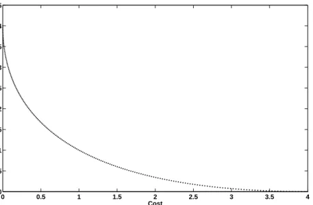
Figure 2.1: An example of a MOP with two objective functions: Cost and Efficiency .

the Pareto front. A sample Pareto front is shown in the Fig. ??. The Pareto front or trade-off surface is delineated by a curved surface.

Although single objective optimization problems may have a unique optimal solution, MOPs usually have a possibly uncountable set of solutions on a Pareto front. Each solution associated with a point on than Pareto front is a vector whose components represent trade-offs in the decision space or Pareto solution space.

Figure 2.2: MOP Evaluation Mapping

The MOPs evaluation function, f : Ω _{→ ∧}, maps decision variables (x= x1, . . . , xn)

to the vectors (y = a1, . . . , ak). This situation is represented in Fig. ?? for the case

n= 2, m= 0, andk = 3. This mapping may or may not be onto some region of objective 11

(25)

function space, dependents upon the functions and constraints composing the particular MOP.

Note that the DM is often selecting solution via choice of acceptable objective per-formance, represented by the Pareto front. Choosing an MOP solution that optimizes only one objective may well ignore solutions, which from an overall standpoint, are “bet-ter”. The Pareto optimal set contains those better solutions. Identifying a set of Pareto optimal solutions is thus key for a DM’s selection of a “compromise” solution satisfying the objectives as “best” possible. Of course, the accuracy of the decision marker’s view depends on both the true Pareto optimal set and the set presented as Pareto optimal.

2.3 Summary

This chapter contains the basic definitions and formal notation that are adopted through-out this thesis. Formal definitions of the general multi-objective optimization and the concept of Pareto optimum are provided. Other related concepts such as Pareto optimal set, Pareto front are also introduced.

(26)

Chapter 3

Multiobjective Evolutionary Algorithms

Introduction Nondominated Sorting Genetic Algorithm Multiobjective Particle Swarm Optimization Multiobjective Bacteria Foraging Optimization Summary

(27)

CHAPTER 3 MULTIOBJECTIVE EVOLUTIONARY

ALGORITHMS

3.1 Introduction

Evolutionary algorithms (EA’s) mimic natural evolutionary principles to constitute search and optimization procedures. EA’s are often well-suited for optimization problems in-volving several, often conflicting objectives. Real world engineering optimization prob-lems involve multiple design factors and constraints and consist in minimizing multiple non-commensurable and often competing objectives. In recent years, many evolution-ary techniques for multiobjective optimization have been proposed [3.1]. In this chapter, we will present two popular Multiobjective evolutionary algorithms, Nondominated Sort-ing Genetic Algorithm-II (NSGA-II) [3.4] and Multiobjective Particle Swarm Optimiza-tion (MOPSO) [3.7], and one proposed “Multiobjective Bacteria Foraging OptimizaOptimiza-tion (MOBFO)” algorithm.

3.2 Nondominated Sorting Genetic Algorithm-II

Genetic algorithms (GA’s) are search and optimization procedures that motivated by the principles of natural genetics and natural selection [3.3]. In this section multiobjective optimization problems solved by an evolutionary algorithm, called Nondominated Sort-ing Genetic Algorithm [3.2, 3.4]. It is a fast nondominated sortSort-ing approach with low computational complexity. It’s come in to category of Elitist multiobjective evolutionary algorithm [3.6]. As the name suggest, an elite-preserving operator favors the elites of a

(28)

CHAPTER 3. MULTIOBJECTIVE EVOLUTIONARY ALGORITHMS

population by giving them an opportunity to be directly carried over the next generation. In this way, a good solution found early on in the run will never be lost unless a better solution is discovered.

3.2.1 Fast Nondominated Sorting Approach

The dual objectives in a multiobjective optimization algorithm are maintained by using a fitness assignment scheme which prefers non-dominated solutions. In the fast nondom-ination approach, the population is sorted based on the nondomnondom-ination. Each solution is assigned a fitness (or rank) equal to its nondomination level (1 is the best level, 2 is the next-best level, and so on). For the population size of N and for M objective functions, in the following paragraph we describe a fast non-dominated sorting approach [3.4].

First, for each solution we calculate two entities:

1) Domination count, np the number of solutions which dominate the solution, and

2) Sp, a set of solutions which the solution pdominates.

An Nondominated Sorting Approach:

Step 1 For each solution p _∈P, np = 0 and initialize Sp = Φ. For all q 6= p and q ∈ P,

perform Step 2 and then proceed to step 3.

Step 2 Ifpq, updateSp =Sp∪q. Otherwise, if qp, set np =np+ 1.

Step 3 If np = 0, keep p in the first non-dominated front F1. Set a front counter i= 1.

Step 4 While Fi 6= Φ, perform the following steps.

Step 5 Initialize Q = Φ for storing next non-dominated solutions. For each p_∈ Pi and

for each q _∈Sp,

Step 5a Update nq =nq−1.

Step 5b Ifnq= 0, keep q inQ, or perform Q=Q∪ {q}.

Step 6 Set i=i+ 1 andFi =Q. Go to step 4.

Steps 1 to 3 find the solutions in the first non-dominated front and require O(M N2₎

computational complexity. Steps 4 to 6 repeatedly find higher fronts and require at most

O(N2_{) comparisons.}

3.2.2 Diversity Preservation

It is desired that an EA maintains a good spread of solutions in the obtained set of solutions. In the proposed MOGA, with a crowded-comparison approach that eliminates the above difficulty to some extent.

(29)

Figure 3.1: Crowding-distance Calculation

Density Estimation

To get an estimate of the density of solutions surrounding a particular solution in the population, we calculate the average distance of two points on either side of this point along each of the objectives. In Fig. ??, the crowding distance of the ith _{solution in its}

front is the average side length of the cuboid (shown with a dashed box).

The algorithm as shown below outlines the crowding-distance computation procedure of all solutions in a nondominated setI.

Step 1: Call the number of solution in I as l = _|I_|. For each solution i in the set, first assign di = 0.

Step 2: For each objective function m = 1,2, . . . , M, sort the set in worse order of

fm or, find the sorted indices vector: Im =sort(fm, >).

Step 3: For m = 1,2, . . . , M, assign a large distance to the boundary solutions, or

dIm

1 =dI

m

l =∞, and for all other solutions j = 2 to (l−1), assign

dIm j =dIjm+ (f Im j+1 m −f Im j−1 m )/(f_mmax−f_mmin) (3.1)

The index Ij denotes the solution index of the j-th member in the sorted list and the

parameters fmax

m and fmmin are the maximum and minimum values of the mth objective

function.

A solution with a smaller value of this distance measure is, in some sense, more crowded by other solutions. This is exactly what we compare in the proposed crowded-comparison operator, described below.

Crowded-Comparison Operator

The crowded-comparison operator (n) guides the selection process at the various stages

(30)

individuali in the population has two attributes: 1) Nondomination rank (irank)

2) Crowding distance (idistance)

We now define a partial order as:

(inj)

(

if (irank < jrank)

or (irank =jrank)

That is, between two solutions with differing nondomination ranks, we prefer the solution with the lower (better) rank. Otherwise, if both solutions belong to the same front, then we prefer the solution that is located in a lesser crowded region.

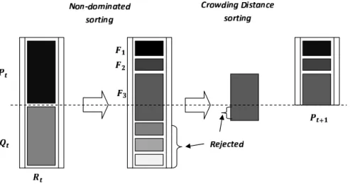
Figure 3.2: NSGA Procedure

3.2.3 Main Loop

Initially, a random parent population P0 is created. The population is sorted in to

dif-ferent non-domination levels. Each solution is assigned a fitness (or rank) equal to its non-domination level (1 is the best level, 2 is the next-best level, and so on). Thus, mini-mization of fitness is assumed. Binary tournament selection (with a crowded tournament operator), recombination, and mutation operators [3.5] are used to create an offspring population Q0 of size N. The NSGA-II procedure is outlined in the following (Fig. ??):

Step 1: Combined population and offspring and create Rt =Pt∪Qt. Perform a

non-dominated sorting to Rt and identify different non-dominated fronts Fi, i= 1, . . . ,etc.

Step 2: Set new population Pt+1 =φ. Set a counter i = 1. Until |Pt+1|+|Fi|< N,

perform Pt+1 =Pt+1+Fi and i=i+ 1.

Step 3: Perform the Crowding-sort (Fi,n) procedure and include the most widely

(31)

spread (N _{− |}Pt+1|) solutions by using the crowding distance values in the sorted Fi to

Pt+1.

Step 4: Create offspring populationQt+1 fromPt+1 by using the crowded tournament

selection, crossover and mutation operators.

3.3 Multiobjective Particle Swarm Optimization

Multiobjective Particle Swarm Optimization (MOPSO), an approach in which Pareto dominance is incorporated into particle swarm optimization (PSO) in order to allow this heuristic to handle problems with several objective functions. Here it uses a secondary (i.e., external) repository of particles that is later used by other particles to guide their own flight.

Kennedy and Eberhart [3.8] initially proposed the swarm strategy for optimization. Particle swarm optimization (PSO) is a stochastic optimization technique that draws inspiration from the behavior of a flock of birds or the collective intelligence of a group of social insects with limited individual capabilities. In PSO, individuals, referred to as particles, are “flown” through hyper dimensional search space. Changes to the position of the particles within the search space are based on the social psychological tendency of individuals to emulate the success of other individuals. A swarm consists of a set of particles, where each particle represents a potential solution. The position of each particle is changed according to its own experience and that of its neighbors. PSO has been found to be successful in a wide variety of optimization tasks [3.8], but until recently it had not been extended to deal with multiple objectives. PSO seems particularly suitable for multiobjective optimization mainly because of the high speed of convergence that the algorithm presents for single objective optimization [3.8]. Here, we represent, called “multiobjective particle swarm optimization” (MOPSO), which allows the PSO algorithm to be able to deal with multiobjective optimization problems [3.7]. These are precisely the main motivations that led us to apply PSO for multiobjective problems [3.10].

3.3.1 Description of the Algorithm

PSO using a Pareto ranking scheme [3.11] could be the straightforward way to extend the approach to handle multiobjective optimization problems. The historical record of best solutions found by a particle (i.e., an individual) could be used to store nondominated solutions generated in the past (this would be similar to the notion of elitism used in evolutionary multiobjective optimization). The use of global attraction mechanisms com-bined with a historical archive of previously found nondominated vectors would motivate

(32)

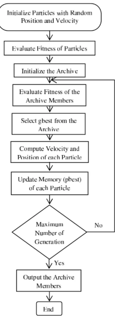
convergence toward globally nondominated solutions. Flow-chart of the MOPSO is shown in Fig. ??.

Figure 3.3: MOPSO Flow Chart

3.3.2 Main Algorithm

The algorithm of MOPSO is the following. 1) Initialize the population pop.

2) Initialize the speed of each particle vel. 3) Evaluate each of the particles in pop.

4) Store the positions of the particles that represent nondominated vectors in the reposi-tory rep.

5) Generate hyper cubes of the search space explored so far, and locate the particles using these hyper cubes as a coordinate system where each particle’s coordinates are defined according to the values of its objective functions.

6) Update the memory of each particle (this memory serves as a guide to travel through

(33)

the search space. This memory is also stored in the repository). 7) WHILE maximum number of cycles has not been reached.

DO

a) Compute the speed of each particle using the following expression:

vel[i] =w_∗vel[i] +r1∗(pbest[i]−pop[i]) +r2∗(rep[h]−pop[i]) (3.2)

where w represents inertia weight, r1 and r2 are random numbers in the range [0,1],

pbest[i] is the best position that the particle i has had, rep[h] is a global best position

that is taken from the repository, the index h is selected in the following way: those hyper cubes containing more than one particle are assigned a fitness equal to the result of dividing any number x >1 by the number of particles that they contain. This aims to decrease the fitness of those hyper cubes that contain more particles and it can be seen as a form of fitness sharing. Then, we apply roulette-wheel selection using these fitness values to select the hypercube from which we will take the corresponding particle. Once the hypercube has been selected, we select randomly a particle within such hypercube.

pop[i] is the current value of the particle i.

b) Compute the new positions of the particles adding the speed produced from the previous step

pop[i] =pop[i] +vel[i] (3.3)

c) Maintain the particles within the search space in case they go beyond their bound-aries (avoid generating solutions that do not lie on valid search space). When a decision variable goes beyond its boundaries, then we do two things: 1) the decision variable takes the value of its corresponding boundary (either the lower or the upper boundary) and 2) its velocity is multiplied by (₋1) so that it searches in the opposite direction.

d) Evaluate each of the particles in pop.

e) Update the contents rep of together with the geographical representation of the particles within the hyper cubes. This update consists of inserting all the currently nondominated locations into the repository. Any dominated locations from the repository are eliminated in the process. Since the size of the repository is limited, whenever it gets full, we apply a secondary criterion for retention: those particles located in less populated areas of objective space are given priority over those lying in highly populated regions.

f) When the current position of the particle is better than the position contained in its memory, the particle’s position is updated using

(34)

The criterion to decide what position from memory should be retained is simply to apply Pareto dominance (i.e., if the current position is dominated by the position in memory, then the position in memory is kept, otherwise, the current position replaces the one in memory, if neither of them is dominated by the other, then we select one of them randomly).

g) Increment the loop counter 8) END WHILE

3.3.3 External Repository

External repository (or archive) is to keep a historical record of the nondominated vectors found along the search process [3.8].It consists of two main parts: the archive controller and the grid.

Figure 3.4: Archive Controller

The Archive Controller

In this approach, archive controller is decide whether a certain solution should be added to the archive or not. The decision-making process is the following:

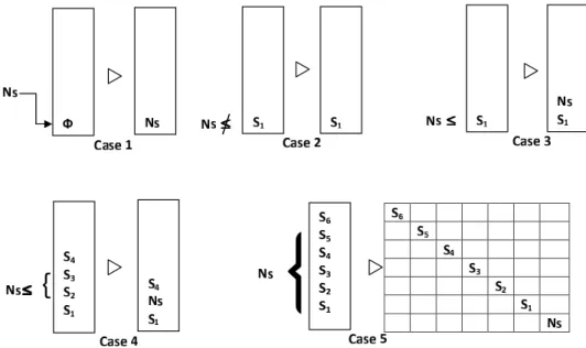
The nondominated vectors found at each iteration in the primary population of our algorithm are compared (on a one-per-one basis) with respect to the contents of the external repository which, at the beginning of the search will be empty. If the external archive is empty, then the current solution is accepted (see case 1, in Fig. ??). If this new solution is dominated by an individual within the external archive, then such a solution

(35)

is automatically discarded (see case 2, in Fig. ??). Otherwise, if none of the elements contained in the external population dominates the solution wishing to enter, then such a solution is stored in the external archive. If there are solutions in the archive that are dominated by the new element, then such solutions are removed from the archive (see cases 3 and 4, in Fig. ??). Finally, if the external population has reached its maximum allowable capacity, then the adaptive grid procedure is invoked (see case 5, in Fig. ??).

Figure 3.5: Adaptive Grid

The Grid

For the diversity preservation of the solutions, our approach uses a variation of the adap-tive grid proposed in [3.8]. All the solutions that are nondominated with respect to the contents of the archive, stored in the external archive. Into the archive, objective function space is divided into regions as shown in Fig. ??. The adaptive grid is a space formed by hyper cubes, have as many components as objective functions. Note that if the individual inserted into the external population lies outside the current bounds of the grid, then the grid has to be recalculated and each individual within it has to be relocated . The main advantage of the adaptive grid is that its computational cost is lower than niching [3.8, 3.11]. In such a case, the computational complexity of the adaptive grid would be the same as niching [i.e., O(N2_)].

3.4 Multiobjective Bacteria Foraging Optimization

The social foraging behavior of Escherichia coli bacteria has been used to solve opti-mization problems [3.12]. In the last decade, approaches based on Bacteria Foraging Optimization (BFO) have received increased attention from the academic and indus-trial communities for dealing with optimization problems that have been shown to be

(36)

intractable using conventional problem solving techniques. Natural selection tends to eliminate animals with poor foraging strategies through methods for locating, handling, and ingesting food and favors the propagation of genes of those animals that have success-ful foraging strategies, since they are more likely to obtain reproductive success [3.13]. After many generations, poor foraging strategies are either eliminated or re-structured into good ones. Since a foraging organism/animal takes actions to maximize the energy utilized per unit time spent foraging, considering all the constraints presented by its own physiology, such as sensing and cognitive capabilities and environmental parameters (e.g., density of prey, risks from predators. physical characteristics of the search area), natural evolution could lead to optimization.

It is essentially this idea that could be applied to Multi-objective optimization prob-lems. The optimization problem search space could be modeled as a social foraging environment where groups of parameters communicate cooperatively for finding solutions to difficult engineering problems.

3.4.1 Bacterial Foraging

Bacteria have the tendency to gather to the nutrient-rich areas by an activity called chemotaxis. It is known that bacteria swim by rotating whip like flagella driven by a reversible motor embedded in the cell wall. E. coli has 8-10 flagella placed randomly on a cell body. When all flagella rotate counterclockwise, they form a compact, helically propelling the cell along a helical trajectory, which is called run. When the flagella rotate clockwise, they pull on the bacterium in different directions, which causes the bacteria to tumble. A brief outline of each of these processes is given in this section.

(1) Chemotaxis: An E. coli bacterium can move in two different ways; it can run (swim for a period of time) or it can tumble, and alternate between these two modes of operation in the entire lifetime. In the BFO, a unit walk with random direction represents a tumble and a unit walk with the same direction in the last step indicates a run. In computational chemotaxis, the movement of theith_{bacterium after one step is represented}

as

θi(j+ 1, k, l) =θi(j, k, l) +C(i)∆(j) (3.5)

where θi₍_{j, k, l}_{) denotes the}_it_h _{bacterium at}_jth _chemotactic, _kth _{reproductive and}_lth

elimination and dispersal. C(i) is the length of unit walk, which is a constant in basic BFO and ∆(j) is the direction angle of the jth _{step. When its activity is run, ∆(}_j_{) is}

same as ∆(j₋1) , otherwise, ∆ is a random angle directed within a range of [0,2π]. If the cost atθi₍_j₊₁_{, k, l}_{) is better than the cost at}_θi₍_{j, k, l}_{), then the bacterium takes}

(37)

another step of size C(i) in that direction otherwise it is allowed to tumble. This process is continued until the number of steps taken is greater than the number of chemotactic loop,Nc .

(2) Reproduction: After allNc chemotactic steps have been covered, a reproduction

step takes place. The fitness values of the bacteria are sorted in ascending order. The lower half of the bacteria having higher fitness die and the remaining Sr =S/2 bacteria

are allowed to split into two identical ones. Thus the population size after reproduction is maintained constant.

(3) Elimination and Dispersal: Since bacteria may stuck around the initial or local optima positions, it is required to diversify the bacteria either gradually or suddenly so that the possibility of being trapped into local minima is eliminated. The dispersion operation takes place after a certain number of reproduction process. A bacterium is chosen, according to a preset probability ped , to be dispersed and moved to another

position within the environment. These events may help to prevent the local minima trapping effectively, but unexpectedly disturb the optimization process. The detailed of this concept is presented in [3.13].

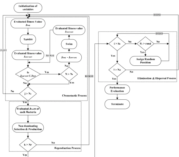
This foraging technique we have applied for the optimization of multiple objectives. Instead of getting single optimal point, in multiobjective optimization large number of nondominated points are the final optimal solutions. The flow chart of the complete algorithm is shown in Fig. ??.

3.4.2 MOBFO Algorithm

The main goal of the BFO based multi-objective algorithm is to find the non-dominated optimum values of the given functionsJ = (f1, . . . , fn). Here, φi(j, k, l) is the position of

a ith _{bacteria in the population of} _N _{at the} _jth _{chemotactic step,} _kth _{reproduction step,}

and lth _elimination

−dispersal event. The main steps of MOBFO given below:

Step 1: Initialize parametersp, N, NC, Ns, Nre, Ned, Ped, C(i), i= (1, . . . , N), φi where,

p: Dimension of the search space,

N: The number of bacteria in the population,

NC: Chemotactic steps,

Nre: The number of reproduction steps,

Ned: The number of elimination−dispersal events,

Ped: Elimination−dispersal with probability,

C(i): The size of the step taken in the random direction specified by the tumble.

Step 2: Elimination₋dispersal loop: l=l+ 1.

Step 3: Reproduction loop: k =k+ 1.

(38)

Figure 3.6: MOBFO Flow-chart

[substep a] Fori= 1,2, ..., N, take a chemotactic step for bacterium i as follows.

[substep b] Compute fitness function,J(i, j, k, l), whereJ = (f1, f2, . . . , fn) set of all

objective functions.

[substep c] LetJlast =J(i, j, k, l) to save this value since we may find a better cost

via a run.

[substep d]Tumble: generate a random vector ∆(i)_{∈ ℜ}p_{with each element ∆}

m(i), m=

1,2, . . . , p, a random number on [₋1,1].

[substep e] Move: Let

φi₍_j_{+ 1}_{, k, l}_{) =}_φi₍_{j, k, l}_{) +}_C₍_i₎_√ ∆(i)

∆T_(i)∆(i)

This results in a step of size C(i) in the direction of the tumble for bacterium i.

[substep f ] Compute J(i, j+ 1, k, l).

[substep g] Swim.

(39)

(i) Let m = 0 (counter for swim length).

(ii) While m < Ns (if have not climbed down too long).

Let m=m+ 1.

If J(i, j+ 1, k, l) Jlast (if dominated), let Jlast =J(i, j+ 1, k, l) and let

φi₍_j_{+ 1}_{, k, l}_{) =}_φi₍_j_{+ 1}_{, k, l}_{) +}_C₍_i₎_√ ∆(i)

∆T_(i)∆(i)

and use this φi₍_j_{+ 1}_{, k, l}_{) to compute the new} _J₍_{i, j}_{+ 1}_{, k, l}_{) as we did in [substep f].}

Else, let m=Ns. This is the end of the while statement.

[substep h] Go to next bacterium (i+ 1) if i ₆=N (i.e., go to [substep b] to process the next bacterium).

Step 5: If j < NC, go to step 3. In this case, continue chemotaxis, since the life of the

bacteria is not over.

Step 6: Reproduction:

[substep a] For the givenk and l, and for each i= 1,2, ..., N, let

Ji

health =Jbesti

whereJi

bestrepresent best fitness value ofithnondominated bacteria according to given

objective functions, which is selected randomly from all nondominated Chemotaxis fitness values of ith _bacteria.

[substep b] Sort bacteria according to nondomination and the crowding distance op-erators. Less crowded bacteria, in objective space, are selected for the reproduction and chemotactic parameters C(i) is find out with [3.14]

C(i) =average Ji health (Ji health+lamda)

where lamdais a constant parameter.

The selected Sr bacteria with the best values split into two bacteria(this process is

performed by the copies that are made are placed at the same location as their parent).

Step 7: If k < Nre, go to [step 3]. In this case, we have not reached the number of

specified reproduction steps, so we start the next generation of the chemotactic loop.

Step 8: Elimination₋dispersal: For i = 1,2, ..., N, with probability Ped, eliminate and

disperse each bacterium, which results in keeping the number of bacteria in the population constant. To do this, if a bacterium is eliminated, simply disperse one to a random location on the optimization domain. If l < Ned, then go to [step 2], otherwise end.

(40)

3.5 Summary

The attractive feature of multiobjective evolutionary algorithms is their ability to find a wide range of nondominated solutions close to the true Pareto optimal solutions. Because of this advantage, the philosophy of solving multiobjective optimization problems can be revolutionized. Evolutionary algorithms process a population of solutions in each iteration, thereby making them ideal candidates for finding multiple trade-off solutions in one single simulation run. In this chapter, we have presented three multiobjective evolutionary algorithms, which can be used to find multiple nondominated solutions close to the Pareto optimal solutions.

(41)

Chapter 4

Performance Evaluation of Multiobjective

Evolutionary Algorithms

Performance Metrics Multiobjective Test Problems Comparison of Multiobjective Evolutionary Algorithms Conclusion

(42)

CHAPTER 4 PERFORMANCE EVALUATION OF

MULTIOBJECTIVE EVOLUTIONARY

ALGORITHMS

When a new and innovative methodology is initially discovered for solving a search and optimization problem, a visual description is adequate to demonstrate the working of the proposed methodology. MOEA’s demonstrated their working by showing the obtained nondominated solutions along with the true Pareto-optimal solutions in the objective space. In these studies, the emphasis has been given to demonstrate how closely the obtained solutions have converged to the true Pareto-optimal front [4.1, 4.2].

4.1 Performance Metrics

With the existence of many different MOEA’s , it is necessary that their performance be quantified on a number of test problems. There are two distinct goals in MOO:

• Discover solutions as close to the Pareto-optimal solutions as possible.

• Find solutions as diverse as possible in the obtained nondominated front.

In some sense, these two goals are orthogonal to each other. The first goal requires a search towards the Pareto-optimal region, while the second goal requires a search along

the Pareto-optimal front, as depicted in Fig. ??. The measure of diversity can also be separated in two different measures ofextent (mean along the spread of extreme solutions) and distribution (meaning the relative distance among solutions).

(43)

CHAPTER 4. PERFORMANCE EVALUATION OF MULTIOBJECTIVE EVOLUTIONARY ALGORITHMS

(a) Two goals for multiobjective opti-mization

(b) Ideal non-dominated solutions

Figure 4.1: Nondominated Pareto Front

Many performance metrics have been suggested [4.1-4.4]. Here, we define two perfor-mance metrics that are more direct in evaluating each of the above two goals in a solution set obtained by a multiobjective optimization algorithm.

4.1.1 Convergence Metric

The first metric Convergence Metric ‘γ’ measures the extent of convergence to a known set of Pareto-optimal solutions [4.3]. Since multiobjective algorithms would be tested on problems having a known set of Pareto-optimal solutions, the calculation of this metric is possible. This metric explicitly computes a measure of the closeness of a set Q of N

solutions from a known set of the True Pareto-optimal setP∗_{. Convergence Metric finds}

an average distance of Qfrom P∗_{, as follows}

γ =

PN i=1di

N (4.1)

where the parameter di is the Euclidean distance (in the objective space) between the

solutioni_∈Q and the nearest member of P∗_:

di = |P∗_| z}|{ min |{z} k=1 v u u t M X m=1 (fm(i)−fm∗(k))2 (4.2)

where fm∗(k) is the mth objective function value of the kth member of P∗.

When all obtained solutions lie exactly on P∗ _{chosen solutions, this metric takes a}

value of zero. In all simulations performed here, we present the averageγ andσγ variance

(44)

4.1.2 Diversity Metric

Although above metric alone can provide some information about the spread in obtained solutions, Deb [4.3] suggested different metric, called Diversity Metric, to measure the spread in solutions obtained by an algorithm directly. The Diversity Metric ‘∆’ measures the extent of spread achieved among the obtained solutions given by:

∆ = PM m=1d e m+ PN i=1|di−d| PM m=1dem+N d (4.3)

wheredi an be any distance measure between neighboring solutions anddis the mean

value of these distance measure. The parameterde

m is distance between the extreme

solu-tions ofP∗ _and_Q _{corresponding to}_mth _{objective function. However, a good distribution}

would make all distances di equal to d and would make df = dl = 0 (with existence of

extreme solutions in the nondominated set). Thus, for the most widely and uniformly spread out set of nondominated solutions, the numerator ∆ of would be zero, making the metric to take a value zero. For any other distribution, the value of the metric would be greater than zero.

4.2 Multiobjective Test Problems

In multi-objective evolutionary computation, researchers have used many different test problems with known sets of Pareto-optimal solutions. For the comparison of the mul-tiobjective algorithms, we choose popular test functions. These test problems are given below.

4.2.1 Schaffer’s (SCH) problem

It is proposed by J. D. Schaffer [4.5]. SCHM inimize:                f1(x) =x2, f2(x) = (x−2)2, −1000_≤x_≤1000.

4.2.2 Kursave(KUR) problem

Our second test function was proposed by Kursawe [4.6]. 31

(45)

CHAPTER 4. PERFORMANCE EVALUATION OF MULTIOBJECTIVE EVOLUTIONARY ALGORITHMS KU RM inimize :                f1(x) = P2 i=1[−10exp(−0.2 p x2 i +x2i+1)], f2(x) = P3 i=1[|xi|0.8+ 5sin(x3i)], −5_≤xi ≤5, i= 1,2,3.

4.2.3 DEB-1 problem

This test problem proposed by the K. Deb. [4.7].

Deb₋1M inimize :                      f1(x) = x1, f2(x) = g(x2)/x1, where g(x2) = 2.0−exp −(x2−0.2 0.004 ) 2 ₋₀_.₈_exp₋₍x2−0.6 0.4 ) 2 0.1_≤x1, x2 ≤1.0.

4.2.4 DEB-2 problem

It is proposed by K.Deb [4.7]. Deb₋2M inimize :                                      f1(x) = x1, f2(x) = g(x1, x2).h(x1, x2), where g(x1, x2) = 11 +x22−10.cos(2πx2), h(x1, x2) = 1− q f1(x1,x2) g(x1,x2) if f1(x1, x2)≤g(x1, x2), otherwise 0 0_≤x1 ≤1,−30≤x2 ≤30.

4.3 Comparison of Multiobjective Evolutionary

Al-gorithms

With the availability of many multiobjective evolutionary algorithms, it is natural to ask which of them (if any) performs better when compared to other algorithms on various test problems. Here, we compare mainly three algorithms, NSGA-II, MOPSO and proposed

(46)

MOBFO, for given test problems which are commonly used. For the following test prob-lems the NSGA-II was run using a population size of 100, a crossover rate of 0.8 (uniform crossover was adopted), tournament selection, and a mutation rate of 0.1. MOPSO used a population of 100 particles, a repository size of 100 particles, a mutation rate of 0.5 and 30 divisions for the adaptive grid. Various parameters used in the simulation study for MOBFO are Sb = 100, Ns = 2, Nc = 4, Nre = 10, Ned = 2−5, Ped = 0.1, C(i) = 0.05

and lamda = 400. These parameters were kept for all the test problems and we only

changed the total number of fitness function evaluations but the same value was adopted for all the algorithms in each of the test problem presented next. In all the following test problems, we report the results obtained from performing 100 independent runs of each algorithm compared.

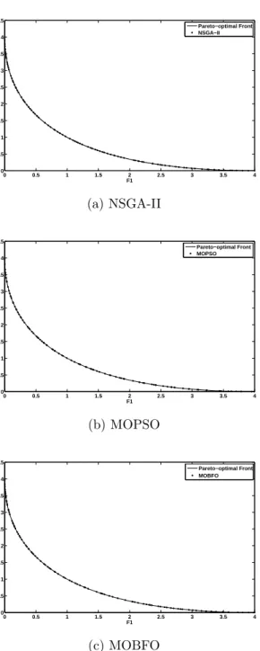
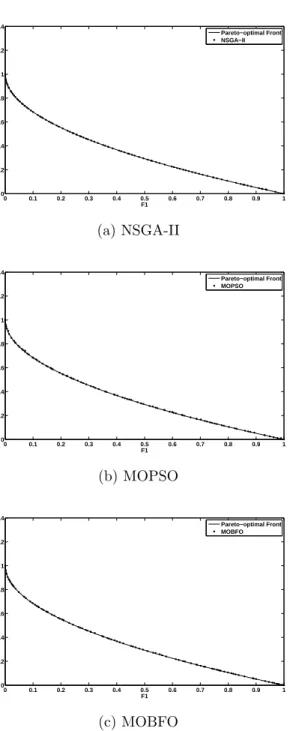
4.3.1 SCH Problem

In this example, the total number of fitness function evaluations was set to 10,000. Fig. ?? show the graphical results produced by our MOBFO,the NSGA-II, and MOPSO in the SCH test function chosen. The true Pareto front of the problem is shown as a continuous line. Tables??, ??and ??shows the comparison of results among the three algorithms considering the metrics previously described. It can be seen that the average performance of MOBFO is slightly below NSGA-II and better than MOPSO with respect to the diversity metric. With respect to convergence metric it places slightly below the NSGA-II and the MOPSO, but with best value than the MOPSO. Also, it is important to notice the very high speed of MOBFO, which requires almost one third of the time than the MOPSO and one tenth of the time than the NSGA-II in this test problem.

Computational Time NSGA-II MOPSO MOBFO

Best 15.40 4.98 1.51

Worst 26.64 6.26 1.96

Mean 17.91 5.57 1.78

Variance 5.6329 0.0820 0.0091

Table 4.1: Computational Time (in sec) required by each Algorithm for the SCH Test Function

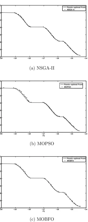
4.3.2 KUR Problem

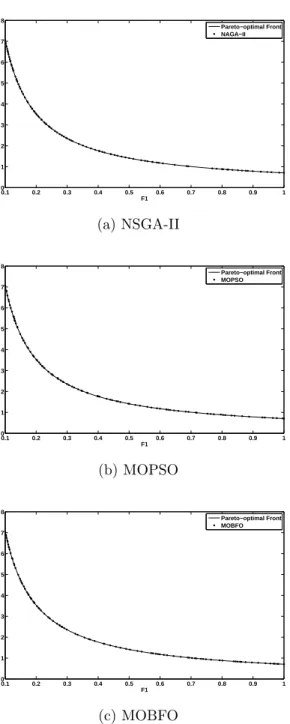
In this example, the total number of fitness function evaluations was set to 20,000. Fig. ?? show the graphical results produced by NSGA-II, the MOPSO, and our MOBFO in the KUR test function chosen. The true Pareto front of the problem is shown

(47)

CHAPTER 4. PERFORMANCE EVALUATION OF MULTIOBJECTIVE EVOLUTIONARY ALGORITHMS 0 0.5 1 1.5 2 2.5 3 3.5 4 0 0.5 1 1.5 2 2.5 3 3.5 4 4.5 F1 F2 Pareto−optimal Front NSGA−II (a) NSGA-II 0 0.5 1 1.5 2 2.5 3 3.5 4 0 0.5 1 1.5 2 2.5 3 3.5 4 4.5 F1 F2 Pareto−optimal Front MOPSO (b) MOPSO 0 0.5 1 1.5 2 2.5 3 3.5 4 0 0.5 1 1.5 2 2.5 3 3.5 4 4.5 F1 F2 Pareto−optimal Front MOBFO (c) MOBFO

Figure 4.2: Nondominated Pareto Front for SCH problem

Convergence Metric NSGA-II MOPSO MOBFO

Best 0.0066 0.0070 0.0068

Worst 0.0089 0.0091 0.0095

Mean 0.0079 0.0079 0.0081

Variance 1.79E-07 1.96e-07 2.31E-07

Table 4.2: Results of the Convergence Metric for the SCH Test Function

Multiobjective Optimization — New Formulation and Application to Radar Signal Processing

Multiobjective Optimization — New Formulation

and Application to Radar Signal Processing

Master of Technology

in

Telematics and Signal Processing

By

VIKAS BAGHEL

Department of Electronics and Communication

National Institute of Technology

Multiobjective Optimization — New Formulation

and Application to Radar Signal Processing

Master of Technology

in

Telematics and Signal Processing

By

VIKAS BAGHEL

Under the Supervision of

Prof. Ganapati Panda

Department of Electronics and Communication

National Institute of Technology

Rourkela, India

2009

National Institute of Technology

CERTIFICATE

Acknowledgment

Vikas Baghel

CONTENTS

Abstract

LIST OF FIGURES

LIST OF TABLES

Chapter 1

Introduction

CHAPTER 1

INTRODUCTION

1.1

Background

1.2

Motivation

1.3

Present Work

1.4

Thesis Organization

Chapter 2

Multiobjective Optimization

CHAPTER 2

MULTIOBJECTIVE OPTIMIZATION

2.1

Introduction

2.2

Definitions

2.2.1

Single Objective Optimization

2.2.2

Multiobjective Optimization

2.3

Summary

Chapter 3

Multiobjective Evolutionary Algorithms

CHAPTER 3

MULTIOBJECTIVE EVOLUTIONARY

ALGORITHMS

3.1

Introduction

3.2

Nondominated Sorting Genetic Algorithm-II

3.2.1

Fast Nondominated Sorting Approach

3.2.2

Diversity Preservation

3.2.3

Main Loop

3.3

Multiobjective Particle Swarm Optimization

3.3.1

Description of the Algorithm

3.3.2

Main Algorithm

3.3.3

External Repository