Network Recasting: A Universal Method for Network Architecture Transformation

(1)

The Thirty-Third AAAI Conference on Artificial Intelligence (AAAI-19)

Network Recasting: A Universal Method

for Network Architecture Transformation

Joonsang Yu, Sungbum Kang, Kiyoung Choi

Dept. of Electrical and Computer Engineering

Neural Processing Research Center (NPRC) Seoul National University, Seoul, Korea

{joonsang.yu, sb05kang}@dal.snu.ac.kr, [email protected]

Abstract

This paper proposes network recasting as a general method for network architecture transformation. The primary goal of this method is to accelerate the inference process through the transformation, but there can be many other practical applica-tions. The method is based on block-wise recasting; it recasts each source block in a pre-trained teacher network to a target block in a student network. For the recasting, a target block is trained such that its output activation approximates that of the source block. Such a block-by-block recasting in a sequential manner transforms the network architecture while preserving the accuracy. This method can be used to transform an ar-bitrary teacher network type to an arar-bitrary student network type. It can even generate a mixed-architecture network that consists of two or more types of block. The network recast-ing can generate a network with fewer parameters and/or ac-tivations, which reduce the inference time significantly. Nat-urally, it can be used for network compression by recasting a trained network into a smaller network of the same type. Our experiments show that it outperforms previous compression approaches in terms of actual speedup on a GPU.

Introduction

Deep Neural Networks (DNNs) are widely used for many kinds of recognition and classification tasks because it has outperformed previous machine learning methods in terms of inference accuracy. New kinds of DNN archi-tecture have been introduced to achieve even higher ac-curacy (Lin, Chen, and Yan 2014; Szegedy et al. 2015; Larsson, Maire, and Shakhnarovich 2017; He et al. 2016; Zagoruyko and Komodakis 2016; Huang et al. 2017), and the networks become deeper and deeper to take the expo-nential advantage of depth (Goodfellow et al. 2016). To train a deep network, He et al. (2016) proposed the residual net-work (ResNet), which consists of the summation of iden-tity mapping and output of convolutional layers. It helps to propagate gradients from top layer to bottom layer, so it can alleviate the vanishing-gradient problem. The densely con-nected network (DenseNet) is also proposed to solve that problem and improve information flow (Huang et al. 2017). DenseNet uses the feature concatenation method instead of summation, so bottom layers can access gradients directly through the concatenation path.

0 2 4 6 8

# multiplications 109 22

23 24 25 26 27 28

validation error (%)

ResNet-34

ResNet-50

ResNet-101

DenseNet-121

DenseNet-169 DenseNet-201

ResNet DenseNet-BC

0 20 40 60

inference time (ms)

22 23 24 25 26 27 28

validation error (%)

ResNet-34

ResNet-50

ResNet-101 DenseNet-121

DenseNet-169

DenseNet-201 ResNet DenseNet-BC

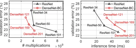
Figure 1: ResNet and DenseNet Top-1 validation errors for different numbers of multiplications (left) and inference times (right). To measure the inference time, single NVIDIA Titan X (Pascal) is used and batch size is set to16. DenseNet has much fewer multiplications than ResNet, but its infer-ence time is much longer.

Deeper network architectures help to achieve higher accu-racy, but those have a huge amount of parameters and com-putation redundancies. To design a compact network archi-tecture, the1×1convolution is added (Szegedy et al. 2015; He et al. 2016; Huang et al. 2017). The additional 1×1 convolution reduces the number of channels of output ac-tivation. The number of parameters and multiplications in the3×3convolution are also reduced thanks to the1×1 convolution. In this reason, bottleneck block in ResNet and dense block in DenseNet use the1×1convolution for the parameter and multiplication reduction.

(2)

layers and thus actual activation load is much larger than the total activation size.

In this paper, we focus on the inference time reduction rather than parameter and multiplication reduction. To re-duce the inference time, we propose the network recast-ing method by transforming the network architecture for smaller activation load. We transform the network architec-ture through block-wise recasting of source blocks into tar-get blocks. The recasting is done by training the tartar-get block to mimic the output activation of the source block, so the accuracy can be preserved after recasting. We can obtain a mixed-architecture networkby recasting parts of the trained network. By the mixed-architecture network, we mean a net-work having multiple types of block that can exploit the ad-vantages of individual block types within a single network. In addition, we can use the network recasting method for network compression by recasting each block to a smaller one of the same type. We have achieved up to3.2×actual speedup with0.22% top-5 accuracy loss on ILSVRC2012 dataset by the DenseNet-121 recasting.

Related Works

Network pruning To reduce the size and inference time of a trained network, several pruning methods such as weight pruning and filter pruning have been proposed. Han et al. (2015) propose an iterative weight pruning method that removes connections and neurons according to the absolute value of parameters. Guo, Yao, and Chen (2016) also pro-pose iterative weight pruning that also gives a chance to re-store connections for pruned weight. However, weight prun-ing methods generate sparse parameter matrices rather than smaller matrices, so its actual speedup is much less than the parameter reduction in general purpose hardware (Liu et al. 2015). The filter pruning methods reduce the size of param-eter and activation matrices after the pruning, so they are more effective to accelerate the inference in any kinds of hardware. To find filters to be pruned, average percentage of zeros (APoZ), sum of absolute values, and reconstruction error of activation are used (Hu et al. 2016; Li et al. 2016; Luo, Wu, and Lin 2017; He, Zhang, and Sun 2017). Luo, Wu, and Lin (2017) find and remove filters that have the smallest influence on the output activation of the next layer, and He, Zhang, and Sun (2017) train a channel pruning mask minimizing the reconstruction error of current output activa-tion and prune the channel of filters according to the trained mask. Liu et al. (2017) and Luo and Wu (2018) use channel scaling factor by adapting additional trainable parameters or squeeze-and-excitation layer (Hu, Shen, and Sun 2018), and then prune filters according to the scaling factor. Recently, Lin et al. (2017) use deep reinforcement learning to select pruning candidates at runtime.

Knowledge distillation To train a smaller network with higher accuracy, mimic learning and knowledge distillation (KD) are introduced by Ba and Caruana (2014) and Hin-ton, Vinyals, and Dean (2014), respectively. These meth-ods train a smaller network called student network using logits of a large network called teacher network. Ba and

Caruana (2014) train a student network by minimizing L2 loss between logits of student and teacher networks. Hin-ton, Vinyals, and Dean (2014) use logits of the teacher network to generate soft target, and train student network by minimizing cross-entropy loss with the soft target. It is hard to train a deep student network due to the vanishing-gradient problem, so several KD methods have been pro-posed to train a deep student network (Romero et al. 2015; Luo et al. 2016). To train a thinner and deeper student net-work using KD, Romero et al. (2015) propose hint train-ing that trains a hidden layer with a convolutional regres-sor. Luo et al. (2016) make additional paths from a hidden layer to the output layer for gradient propagation without vanishing. In addition, Zagoruyko and Komodakis (2017) introduce the attention transfer method to reduce the num-ber of residual blocks while conserving the accuracy. Yim et al. (2017) also propose the residual block reduction method using the relationship between input and output activations. Also, there is a recent research to train the ResNet using log-its of DenseNet (Furlanello et al. 2018).

Key differences Our work is for general recasting of neu-ral networks. It can be used in various ways such as net-work size reduction or netnet-work type transformation. Com-pared to the previous work on network size reduction using weight/filter pruning, our work is different in that the infer-ence process of the reduced network can be made signifi-cantly faster through the reduction of activations. We also reveal the fact that reducing activation size is more important for inference speed than reducing the number of parameters. Compared to other approaches using the knowledge distilla-tion technique, our work is different in that the technique is applied sequentially to further enhance the accuracy.

Network Recasting

The network recasting method recasts a pre-trained network into a network of different type and/or size. Given the pre-trained teacher network, we transform each block (source block) in the teacher network into a new block (target block) of pre-defined type and size in the student network. The transformation is done by training the target block to gen-erate output activations similar to those of the source block. We call this process block recasting. In this process, the source block can be considered as an unknown function, and the target block can be considered as a functional approxi-mator similar to a multilayer perceptron (Hornik 1991). Af-ter recasting all candidate blocks, we obtain the student net-work, which is faster than the teacher network while preserv-ing the functionality or accuracy. We call the entire process network recasting.

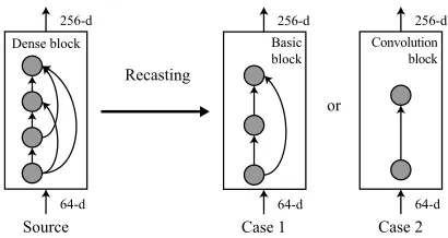
Recasting from DenseNet to ResNet and ConvNet

(3)

Dense block Convolution block

64-d 64-d

256-d 256-d

Source

Basic block

64-d 256-d

Case 1 Case 2

or Recasting

Figure 2: Block recasting of a dense block into a basic block (Case 1) and a convolution block (Case 2). The basic block has shorter inference time than the dense block because it has much smaller activation load. The convolution block is even faster than the basic block, but its capacity is much smaller and so it can cause accuracy loss.

Convolution block

64-d Basic

block

64-d

64-d 64-d

Case 1 Target

Recasting

Bottleneck block

64-d

256-d

1x1 1x1

Case 2 or

Figure 3: Block recasting of a residual block—basic block (Case 1) and bottleneck (Case 2)— into a convolution block. The recasting of the basic block keeps the same number of input and output channels. However, since the bottleneck block uses a smaller number of channels for the feature ex-traction, we recast it into a convolution block that has the same number of input and output channels as the original 3×3convolution.

and shortcut as shown in Figure 2. Even though the ba-sic block has more parameters and multiplications than the dense block, its activation load is much smaller and thus it is much faster. For more inference time reduction, we can recast the dense block into a single convolution block, al-though it can cause more accuracy loss because it has a very small capacity. Figure 2 shows the two examples of recast-ing the first dense block in DenseNet-121.

Recasting from ResNet to ConvNet

Figure 3 illustrates the block recasting of a residual block into a convolution block. In the basic block, local features are extracted from the input activations using3×3filters, and thus, we recast the basic block into a3×3 convolu-tion block. Since the new convoluconvolu-tion block has the same number of filters as the original basic block, the dimension of the output activations is not changed. However, in bottle-neck block recasting, the dimension of the output activation is reduced as shown in Figure 3 (Case 2) for the first bot-tleneck block of ResNet-50. Although the output activation becomes smaller, the number of linearly independent

fea-Table 1: Candidates for the network recasting.

Recasting Type Source Target Dimension

Transformation

Dense Dense Basic Bottleneck

Basic Convolution Convolution Convolution

Preserved Preserved Preserved Reduced

Compression Basic

Convolution

Basic Convolution

Reduced Reduced

tures is not changed because the second1×1convolution in the source block just combines its input activations linearly to extend the dimension of output activation. Therefore, the next block in the student network still can reconstruct simi-lar activation map.

Compression

The network recasting can be used to compress the large network while preserving accuracy. In this case, we assume that the network has redundancy such as ineffectual filters and redundant filters. An ineffectual filter denotes a filter that cannot extract any meaningful feature, and aredundant filter denotes a filter that extracts a feature very similar to the one extracted by some other filter or a feature that can be obtained by combining features from other filters. To re-move those filters, previous approaches use APoZ (Hu et al. 2016), sum of absolute values of a filter (Li et al. 2016), or influence on next activations (Luo, Wu, and Lin 2017; He, Zhang, and Sun 2017) as the criteria, but redundant fil-ters cannot be founded with those approaches. A possible approach is to find such redundant filters by checking the similarity between every pair of filters. However, it requires a huge amount of computations for similarity check and does not guarantee a good result. Instead, we recast a given source block into a smaller target block that has the same type as the source block. Then we train the target block and the next block to reconstruct the output activation of the next block with smaller number of filters. If the next block can recon-struct a similar output activation, the new target block can extract effective features for reconstruction. For example, a convolution block is recast into another convolution block that has a smaller number of filters. Then we train both the new convolution block and the next block to reconstruct the orginal activation map of the source next block. After train-ing, we can obtain a more effective filter set without any similarity or effectiveness check criteria.

Block Training

(4)

64-d 64-d 256-d

64-d 256-d

Next block (rebuilt) Next block

256-d

Target block Source

block

64-d 64-d Target

block

64-d 256-d Source block

Dimension mismatch

Ws*=argmin Lmse(WT, Ws)

Teacher Student Teacher Student

Figure 4: The dimension mismatch happens when the source block is recast into a smaller target block. The next block is used to match the dimension of output activation. After re-building the next block, both blocks are trained by minimiz-ingLmse(WT, WS).

block by approximating the output activations of the next block as shown in Figure 4. The next block is rebuilt from the corresponding source block by reducing the filter size when the target block has a smaller number of channels. Both the target block and the next block are initialized ran-domly and trained to minimize the loss of mean-square error (MSE) between teacher’s and student’s activations given by,

Lmse(WT, WS) = 1

NkA(x;WT)−A(x;WS)k

2 2, (1)

whereA means the activation of the next block, and xis the input data.WT andWS indicate parameters of teacher network and student network, respectively. N denotes the size of an output activation of the next block.

Sequential Recasting and Fine-tuning

To recast the entire network, we apply the block recasting method sequentially. Figure 5 shows an example of sequen-tial recasting method. The type and dimension of the first (target) block of the student network are determined, and then the second block is rebuilt from the second block of the teacher network; if there is no dimension mismatch, the sec-ond block will be the same as that of the teacher network. The two blocks are initialized randomly and trained by min-imizingLmse(WT, WS). Now, the second block becomes the target. Thus, its type and dimension are determined, the third block is rebuilt, and both blocks are initialized ran-domly. To train the second and third blocks, we reuse the trained first block. The first block is already trained in the previous step, but it still has approximation errors. We can reduce the effect of its errors by training both the previous and current blocks. Therefore, three blocks are trained in the second step by minimizing Lmse(WT, WS). This process is continued for the following blocks until the last block is recast as a new block. We can select arbitrary blocks as can-didates for recasting so that the student network can consist of multiple types of block. For example, the student network can have both residual and dense blocks when only the first dense block is recast into a residual block. We call the net-work that has multiple types of block asmixed-architecture

network. The mixed-architecture network can have advan-tages of both blocks. For example, by mixing dense blocks and residual blocks, we can obtain a mixed-architecture net-work that is faster than DenseNet and has fewer parameters than ResNet.

The block-by-block sequential recasting has two advan-tages. First, the functionality of each block is much simpler than that of the whole network. Thus, it is easier to approxi-mate the functionality of each block. By approximating each of easier sub-functions, we can finally obtain the student net-work with smaller approximation error. Secondly, sequen-tial recasting can alleviate the vanishing-gradient problem. When the source block is recast as a convolution block, the student network cannot be trained well due to the gradient vanishing. However, sequential recasting has very short gra-dient paths from the output activation to the target block, so it can be trained well. Therefore, we can obtain the student network with higher accuracy using sequential recasting.

After finishing sequential recasting, we use the knowl-edge distillation approach to fine-tune the student network. There are approximation errors after sequential recasting, and we can reduce the effect of those errors by training the whole network. We train the student network with logits of the teacher network and ground truth. Thus, our knowledge distillation (KD) loss is defined by

Lkd(WT, WS) =Lmse logit(WT, WS) +Lce(ytrue, WS), (2) where Lmse logit is the MSE loss for the logits, and Lce is the cross-entropy loss between the given labelytrueand softmax output of the student network that is parameterized byWs.

Experiments

We conducted several experiments for the network recast-ing. For the experiments, we used CIFAR and ILSVRC2012 dataset and four kinds of network architectures; ResNet (He et al. 2016), Wide ResNet (WRN) (Zagoruyko and Ko-modakis 2016), DenseNet (Huang et al. 2017), and VGG-16 (Simonyan and Zisserman 2015). We adopted batch nor-malization (Ioffe and Szegedy 2015) for all networks, be-cause it was also effective for block-wise training. The net-work recasting was implemented on thePyTorchframework. We used the Xavier initializer (Glorot and Bengio 2010) in all experiments. We used SGD with Nesterov momentum (Sutskever et al. 2013) to train the teacher network and used Adam optimizer (Kingma and Ba 2015) for the network re-casting. In addition, we trained the student network with KD and back propagation from scratch using SGD with Nes-terov momentum for the comparison.

Visualization of Filter Reduction

(5)

64-d 64-d 256-d

64-d 256-d 256-d

512-d 512-d 1000-d

2048-d 2048-d 1000-d

64-d 64-d 256-d

256-d 256-d 256-d

64-d 64-d

Classifier (rebuilt) Classifier

Block 3 (rebuilt) Block 3

Block 2 (rebuilt)

Block 2 _(source)Block 2 Block 2_(target) Block 16_(source) Block 16_(target)

Block 1 (target) Block 1

(source) Block 1 (trained)Block 1

Teacher

Student

Teacher

Student

Teacher

)

Figure 5: An example of sequential recasting for ResNet-50. All blocks are recast in this example. In each step, the target block and the next block (shaded blocks) are initialized randomly and trained by minimizingLmse(WT, WS).

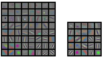
Figure 6: Visualization of filters in the first layer of AlexNet (left) and a student network (right). Redundant filters are re-moved after network recasting.

for eight epochs, and fine-tuned the entire student network; the learning rates for the recasting of the first block and the fine-tuning were0.0005and0.0001, respectively. Every five epochs, the running rates were divided by 10. Figure 6 shows filters extracted from the first layers of the teacher and stu-dent networks. Filters of the teacher network consist of many ineffectual and redundant filters, but those are eliminated as shown in Figure 6. In addition, the student network achieves the top-1 error of 44.20% and the top-5 error of 21.54%. The top-1 and the top-5 errors increase by only0.72% and 0.61%, respectively. Note that it is hard to remove many fil-ters without accuracy loss because AlexNet has a relatively large (11×11) filters. The filter size is related to the di-mension of filter vector, and many more filters are required to span the vector space as the filter size increases. As ex-pected, we could remove many more filters on both VGG-16 and ResNet, which have only3×3filters.

CIFAR

For CIFAR dataset, we used ResNet-56, ResNet-83, WRN-28-10, DenseNet-100, and VGG-16. Especially, ResNet-83 has the same number of blocks with ResNet-56, but consists of bottleneck blocks. In addition, we used a modified ver-sion of VGG16, which has only one hidden fully-connected layer with512neurons. Teacher networks were trained from

scratch using back propagation. We used CIFAR-10 and 100 dataset with the standard data augmentation, which consists of four pixel zero-padding and random cropping, and hori-zontal flipping with0.5probability.

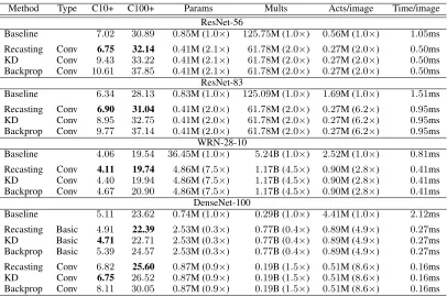
In CIFAR experiments, we recast all blocks of teacher net-works, so there is no mixed-architecture result. We counted the number of parameters, multiplications, and activation loads for the convolution operation. Especially, we reported the activation load of a single image in Table 2. Table 2 shows the architecture transformation results. The network recasting achieved similar accuracy with the teacher net-work, and activation access is reduced significantly. It shows lower test error compared to other methods in all network ar-chitectures. When networks were recast into a plain convolu-tional network, the network recasting achieved much lower test error compared with both KD and back propagation. The sequential recasting can alleviate the vanishing-gradient problem, so its results outperformed the others.

We also compressed the VGG-16 and WRN-28-10 us-ing the network recastus-ing. In this experiment, source blocks were recast into 2.5×and 5× smaller blocks in VGG-16 and WRN-28-10, respectively. Table 3 shows compression results of both networks. The network recasting achieved the smallest accuracy loss compared with other methods. Espe-cially, network recasting achieved1.58% and3.57% lower test error compared with KD and back propagation in VGG-16 compression on CIFAR-100.

(6)

Table 2: Error rates (%) of architecture transform results on CIFAR datasets. (B/M: billion/million)

Method Type C10+ C100+ Params Mults Acts/image Time/image

ResNet-56

Baseline 7.02 30.89 0.85M (1.0×) 125.75M (1.0×) 0.56M (1.0×) 1.05ms

Recasting Conv 6.75 32.14 0.41M (2.1×) 61.78M (2.0×) 0.27M (2.0×) 0.50ms

KD Conv 9.43 33.22 0.41M (2.1×) 61.78M (2.0×) 0.27M (2.0×) 0.50ms

Backprop Conv 10.61 37.85 0.41M (2.1×) 61.78M (2.0×) 0.27M (2.0×) 0.50ms

ResNet-83

Baseline 6.34 28.13 0.83M (1.0×) 125.09M (1.0×) 1.69M (1.0×) 1.51ms

KD Conv 8.95 32.75 0.41M (2.0×) 61.78M (2.0×) 0.27M (6.2×) 0.95ms

WRN-28-10

Baseline 4.06 19.54 36.45M (1.0×) 5.24B (1.0×) 2.52M (1.0×) 0.81ms

Recasting Conv 4.11 19.74 4.86M (7.5×) 1.17B (4.5×) 0.90M (2.8×) 0.41ms

KD Conv 4.40 19.94 4.86M (7.5×) 1.17B (4.5×) 0.90M (2.8×) 0.41ms

Backprop Conv 4.67 20.90 4.86M (7.5×) 1.17B (4.5×) 0.90M (2.8×) 0.41ms

DenseNet-100

Baseline 5.11 23.62 0.74M (1.0×) 0.29B (1.0×) 4.41M (1.0×) 2.12ms

Recasting Basic 4.91 22.39 2.53M (0.3×) 0.77B (0.4×) 0.89M (4.9×) 0.27ms

KD Basic 4.71 22.71 2.53M (0.3×) 0.77B (0.4×) 0.89M (4.9×) 0.27ms

Backprop Basic 5.39 24.57 2.53M (0.3×) 0.77B (0.4×) 0.89M (4.9×) 0.27ms

Recasting Conv 6.82 25.60 0.87M (0.9×) 0.19B (1.5×) 0.51M (8.6×) 0.16ms

KD Conv 6.75 26.52 0.87M (0.9×) 0.19B (1.5×) 0.51M (8.6×) 0.16ms

Backprop Conv 8.11 30.05 0.87M (0.9×) 0.19B (1.5×) 0.51M (8.6×) 0.16ms

Table 3: Error rates (%) of compression results on CIFAR datasets. (B/M: billion/million)

Method Type C10+ C100+ Params Mults Acts/image Time/image

VGG-16

Baseline 6.85 28.80 14.71M (1.0×) 313.20M (1.0×) 0.31M (1.0×) 0.37ms

KD Conv 9.24 33.14 2.36M (6.2×) 50.63M (6.2×) 0.13M (2.4×) 0.31ms

WRN-28-10

Baseline 4.06 19.54 36.45M (1.0×) 5.24B (1.0×) 2.52M (1.0×) 0.81ms

Recasting Basic 5.18 24.13 1.46M (24.9×) 0.21B (24.5×) 0.52M (4.9×) 0.56ms

KD Basic 5.48 25.28 1.46M (24.9×) 0.21B (24.5×) 0.52M (4.9×) 0.56ms

Backprop Basic 5.39 25.78 1.46M (24.9×) 0.21B (24.5×) 0.52M (4.9×) 0.56ms

ILSVRC2012

For ILSVRC2012 dataset, we used the pre-trained ResNet-50, DenseNet-121, and VGG-16 available from torchvi-sion which is one of the PyTorch packages. These pre-trained networks were used as the teacher networks. We recast the blocks of ResNet-50 into convolution blocks, and the blocks of DenseNet-121 into basic blocks. In ad-dition, we recast only parts of these networks to obtain mixed-architecture networks. In Table 4,Recasting(C) indi-cates that the student network only has convolution blocks, and Recasting(C+Rbt) denotes that the student network has both convolution and bottleneck blocks. In the same way,Recasting(Rbs)andRecasting(Rbs+D)denotes that the student networks consist of only basic blocks and both basic blocks and dense blocks, respectively. KD(C+Rbt) and KD(Rbs+D) have the same network architecture as

Recasting(C+Rbt) and Recasting(Rbs+D) respectively, but those are trained with only KD method. For the VGG-16 compression, we used two criteria: higher parameter reduc-tion (Recasting(C P)) and higher activation reduction ( Re-casting(C A)). In addition, we measured the actual inference time for all networks on an NVIDIA Titan X (Pascal) GPU, and batch sizes were set to 1 and 64.

(7)

Table 4: Error rate (%) of network recasting results on ILSVRC2012. (B/M: billion/million)

Method Top1 Top5 Params Mults Acts/image Time/image Time/bacth ResNet-50

Baseline 23.85 7.13 25.50M 4.09B 11.57M 6.16ms 107.17ms

Recasting(C) 30.74 10.39 10.29M 1.71B 2.53M 2.12ms 37.21ms Recasting(C+Rbt) 25.00 7.71 21.72M 2.40B 3.69M 3.79ms 49.97ms KD(C+Rbt) 27.00 8.30 21.72M 2.40B 3.69M 3.79ms 49.97ms

DenseNet-121

Recasting(Rbs) 26.42 8.25 32.23M 8.15B 5.32M 3.95ms 81.17ms Recasting(Rbs+D) 24.87 7.59 10.42M 5.72B 9.15M 9.40ms 88.94ms KD(Rbs+D) 24.90 7.65 10.42M 5.72B 9.15M 9.40ms 88.94ms

VGG-16

Recasting(C P) 28.25 9.41 81.93M 4.73B 8.27M 3.45ms 116.45ms Recasting(C A) 30.05 10.38 120.61M 3.12B 3.30M 3.61ms 63.52ms

Table 5: Comparison of error rate (%) with previous works on ILSVRC2012. (B/M: billion/million)

Method Top1 Top5 Params Mults Acts/batch Actual speed-up

ResNet-50

Recasting(C+Rbt) 25.00 7.71 21.72M 2.40B 236.16M 2.1×

ThiNet-30 (Luo, Wu, and Lin 2017) 31.58 11.7 8.66M 1.10B - 1.3× AutoPruner (r= 0.3) (Luo and Wu 2018) 27.47 8.89 - 1.32B -

-VGG-16

Recasting(C A) 30.05 10.38 120.61M 3.12B 220.61M 3.2×

ThiNet-Conv (Luo, Wu, and Lin 2017) 30.20 10.47 131.44M 4.79B - 2.5×

RNP (3×) (Lin et al. 2017) - 12.42 - - - 2.3×

Channel Pruning (3×) (He, Zhang, and Sun 2017) - 11.10 - - - 2.5× AutoPruner (r= 0.4) (Luo and Wu 2018) 31.57 11.57 - 4.09B -

-training time for a deep network and shorter -training time with similar accuracy for a shallow network.

As shown in Table 4, the network recasting signifi-cantly reduced the inference time in all experiments. Re-casting(C) and Recasting(Rbs) achieved2.9×and3.2× in-ference time reduction for a single image compared with original ResNet-50 and DenseNet- 121, respectively. More-over, mixed-architecture networks also achieved significant inference time reduction with smaller accuracy loss. For the batch processing, Recasting(C+Rbt) achieved2.1×time reduction with 0.58% top-5 accuracy loss compared to Baseline, and Recasting(Rbs+D) achieved 1.3× time re-duction even with 0.44% higher top-5 accuracy. In par-ticular, Recasting(Rbs+D) achieved similar accuracy and inference time with 3.1× fewer parameters compared to Recasting(Rbs). In VGG-16 compression, Recasting(C P) and Recasting(C A) achieved1.7×parameter reduction and 4.6×activation reduction with0.91% and2.05% top-5 ac-curacy loss, respectively. Recasting(C A) achieved3.2× in-ference time reduction compared to the baseline.

We compared our results with several previous ap-proaches (Luo, Wu, and Lin 2017; He, Zhang, and Sun 2017; Lin et al. 2017; Luo and Wu 2018). For the comparison, we

used batch inference time because previous approaches have reported inference time only for the batch processing. Ta-ble 5 shows that the network recasting achieved much higher inference time reduction. In ResNet-50, Recasting(C+Rbt) achieved lower error rate and much higher actual speedup compared with ThiNet (Luo, Wu, and Lin 2017). ThiNet only reduced filters and multiplications in3×3convolution of bottleneck blocks, so it cannot accelerate the inference ef-fectively because activation load is still large. However, the network recasting can reduce the activation load effectively, so it achieved 2.1×actual speedup with smaller accuracy loss. Luo and Wu (2018) does not mention actual-speedup, but we can guess that our network recasting result is much faster than their AutoPruner result because they cannot re-move the1×1convolution. For the VGG-16 compression, the network recasting also achieves much higher speedup with lower error rate compared to previous approaches. It also achieves higher parameter and multiplication reduction with similar accuracy compared to others.

Conclusion

(8)

method can accelerate network inference by transforming the network (teacher) to a more efficient one (student). We could recast residual and dense blocks into convolution and residual blocks, respectively, to achieve much higher ac-tual speedup at small accuracy loss. By recasting blocks sequentially, the student network can be trained well even though there is no shortcut or dense connection. In addition, our method can recast arbitrary blocks, thereby producing a mixed-architecture network. The mixed-architecture net-works produced as such achieved2.1×inference time with 0.58% top-5 accuracy loss compared to original ResNet-50, and also achieved1.3×inference time reduction with0.44% higher top-5 accuracy on DenseNet-121 recasting. We also applied the network recasting for the purpose of compres-sion and achieved higher comprescompres-sion ratio and speedup compared to previous approaches. Our method can be ap-plied to various kinds of network architecture to transform it into various kinds of target network architecture.

Acknowledgments

This work was supported by Samsung Advanced Institute of Technology.

References

Ba, J., and Caruana, R. 2014. Do deep nets really need to be deep? InNIPS, 2654–2662.

Furlanello, T.; Lipton, Z. C.; Amazon, A.; Itti, L.; and Anandkumar, A. 2018. Born again neural networks. In ICML, 1607–1616.

Glorot, X., and Bengio, Y. 2010. Understanding the diffi-culty of training deep feedforward neural networks. In AIS-TATS, 249–256.

Goodfellow, I.; Bengio, Y.; Courville, A.; and Bengio, Y. 2016.Deep learning, volume 1. MIT press Cambridge. Guo, Y.; Yao, A.; and Chen, Y. 2016. Dynamic network surgery for efficient DNNs. InNIPS, 1379–1387.

Han, S.; Pool, J.; Tran, J.; and Dally, W. 2015. Learning both weights and connections for efficient neural network. InNIPS, 1135–1143.

He, K.; Zhang, X.; Ren, S.; and Sun, J. 2016. Deep residual learning for image recognition. InCVPR, 770–778.

He, Y.; Zhang, X.; and Sun, J. 2017. Channel pruning for accelerating very deep neural networks. In ICCV, 1389– 1397.

Hinton, G.; Vinyals, O.; and Dean, J. 2014. Distilling the knowledge in a neural network. InNIPS Deep Learning and Representation Learning Workshop.

Hornik, K. 1991. Approximation capabilities of multilayer feedforward networks.Neural networks4(2):251–257. Hu, H.; Peng, R.; Tai, Y.-W.; and Tang, C.-K. 2016. Net-work trimming: A data-driven neuron pruning approach to-wards efficient deep architectures. arXiv preprint arXiv: 1607.03250.

Hu, J.; Shen, L.; and Sun, G. 2018. Squeeze-and-excitation networks. InCVPR, 7132–7141.

Huang, G.; Liu, Z.; Weinberger, K. Q.; and van der Maaten, L. 2017. Densely connected convolutional networks. In CVPR, 4700–4708.

Ioffe, S., and Szegedy, C. 2015. Batch normalization: Accel-erating deep network training by reducing internal covariate shift. InICML, 448–456.

Kingma, D. P., and Ba, J. 2015. Adam: A method for stochastic optimization. InICLR.

Larsson, G.; Maire, M.; and Shakhnarovich, G. 2017. Frac-talnet: Ultra-deep neural networks without residuals. In ICLR.

Li, H.; Kadav, A.; Durdanovic, I.; Samet, H.; and Graf, H. P. 2016. Pruning filters for efficient convnets. InICLR. Lin, J.; Rao, Y.; Lu, J.; and Zhou, J. 2017. Runtime neural pruning. InNIPS, 2181–2191.

Lin, M.; Chen, Q.; and Yan, S. 2014. Network in network. InICLR.

Liu, B.; Wang, M.; Foroosh, H.; Tappen, M.; and Pensky, M. 2015. Sparse convolutional neural networks. InCVPR, 806–814.

Liu, Z.; Li, J.; Shen, Z.; Huang, G.; Yan, S.; and Zhang, C. 2017. Learning efficient convolutional networks through network slimming. InICCV, 2755–2763.

Luo, J.-H., and Wu, J. 2018. AutoPruner: An end-to-end trainable filter pruning method for efficient deep model in-ference.arXiv preprint arXiv: 1805.08941.

Luo, P.; Zhu, Z.; Liu, Z.; Wang, X.; and Tang, X. 2016. Face model compression by distilling knowledge from neurons. InAAAI, 3560–3566.

Luo, J.-H.; Wu, J.; and Lin, W. 2017. ThiNet: A filter level pruning method for deep neural network compression. In ICCV, 5058–5066.

Romero, A.; Ballas, N.; Kahou, S. E.; Chassang, A.; Gatta, C.; and Bengio, Y. 2015. FitNets: Hints for thin deep nets. InICLR.

Simonyan, K., and Zisserman, A. 2015. Very deep convolu-tional networks for large-scale image recognition. InICLR. Sutskever, I.; Martens, J.; Dahl, G.; and Hinton, G. 2013. On the importance of initialization and momentum in deep learning. InICML, 1139–1147.

Szegedy, C.; Liu, W.; Jia, Y.; Sermanet, P.; Reed, S.; Anguelov, D.; Erhan, D.; Vanhoucke, V.; and Rabinovich, A. 2015. Going deeper with convolutions. InCVPR, 1–9. Yim, J.; Joo, D.; Bae, J.; and Kim, J. 2017. A gift from knowledge distillation: Fast optimization, network mini-mization and transfer learning. InCVPR, 4133–4141. Zagoruyko, S., and Komodakis, N. 2016. Wide residual networks. InBMVC, 87.1–87.12.