SIMILARITY MEASURE OF INTERVAL VALUED VAGUE SETS TO MULTIPLE ATTRIBUTE DECISION MAKING

Volume 2, Issue 4, April 2013

Page 318

ABSTRACT

In real life, a person may observe that an object belongs and not belongs to a set to certain degree, but it is possible that he is not sure about it. In other words, there may be some hesitation or uncertainty about the membership and non-membership degree of an object belonging to a set. In fuzzy set theory there is no means to incorporate that hesitation in membership degree. A possible solution is to use vague sets and the concept of vague set was proposed by Gau and Buehrer [1993]. Distance measure between vague sets is one of the most important technologies in various application fields of vague sets. But these methods are unsuitable to deal with the similarity measures of IFSs. In this paper we have extended the work of Zeshui Xu [2007] and also proposed a method to develop some similarity measure of interval valued vague sets and define the positive and negative ideal of interval valued vague sets, and apply the similarity measures to multiple attribute decision making based on vague information. A numerical example is also given to elaborate our technique.

Keywords- Vague sets; Fuzzy sets; Intuitionstic Fuzzy Sets (IFS); Membership function; Distance measure; Interval

Valued Vague Sets; Similarity Measure; Decision Making

1.

INTRODUCTION

Atanassov (1986) defined the notion of intuitionstic fuzzy sets, which is a generalization of notion of Zadeh’s fuzzy set which was later on called vague set the concept given by Gau and Buehrer (1993), which is characterized by a membership function and a non membership function. The concept of vague set is the generalization of the fuzzy set which introduced by Zadeh (1965), and has also been found to be very highly useful to deal with vagueness. In less than two decades since its first appearance, the IFS theory has been investigated by many authors (Atanassov & Georgiev , 1993; Bustince et al.,2000; De et al ., 2001; Deschrijver & Kerre, 2003; Grzegorzewski, 2004; Mondal & Samanta, 2001,2002; Szmidt & Kacprzyk, 2000,2001), and has been applied in different fields, including decision making ( Atanassov, Pasi & Yager, 2005; Chen and Tan.1994; Hong & Choi, 2000; Szmidt & Kacprzyk, 2002; Xu & Ronald, 2006), logic programming ( Atanassov & Georgiev, 1993), medical diagnosis ( De et al., 2001), etc Gau & Buehrer (1993) defined the concept of vague set. Bustine & Burillo (1996) showed that the notion of vague set coincides with that of IFS. De et al., 2000 defined concentrated IFS, dilated IFS, normalization of IFS, and made some characterization. Atanassov & Georgiev (1993) presented a logic programming system which uses a theory of IFSs to model various forms of uncertainty. Bustince et al (2000) proposed some definitions of distances between IFSs and compared them with the approach used for fuzzy sets. Szmidt & Kacprzyk (2001) introduced a measure of entropy for IFS. Mondal and Samanta (2001) defined the topology of interval valued IFSs. Mondal and Samanta (2002) established an intuitionistic fuzzy topological space. Deschrijver & Kerre (2003) presented an intuitionistic fuzzy version of triangular compositions and investigated some properties of these compositions, such as containment, convertibilitry, monotonicity, interaction with union and intersection. Many methods have been proposed for measuring the degree of similarity between fuzzy sets.

In real life, a person may observe that an object belongs and not belongs to a set to certain degree, but it is possible that he is not sure about it. In other words, there may be some hesitation or uncertainty about the membership and non-membership degree of an object belonging to a set. In fuzzy set theory there is no means to incorporate that hesitation in membership degree. A possible solution is to use vague sets and the concept of vague set was proposed by Gau and Buehrer [1993]. But these methods are unsuitable to deal with the similarity measures of IFSs.

In this paper we have extended the work of Zeshui Xu [2007] and also proposed a method to develop some similarity measure of interval valued vague sets and define the positive and negative ideal of interval valued vague sets, and apply the similarity measures to multiple attribute decision making based on vague information.

SIMILARITY MEASURE OF INTERVAL

VALUED VAGUE SETS TO MULTIPLE

ATTRIBUTE DECISION MAKING

M. K. Sharma1, 2Rajesh Dangwal, 2Vintesh Sharma and 3Vinesh Kumar

1

Department of Mathematics, R.S.S. (PG), Pilkhuwa, (Hapur), India

2

H.N.B. Garhwal University, Campus Pauri (U.K)

3

Volume 2, Issue 4, April 2013

Page 319

2. SOME DEFINITIONS:

2.1: Definition: An interval valued fuzzy sets

A

over a universe of discourse

X

is defined by a function

:

([0,1]),

A

T

X

D

where D ([0, 1]) is the set of all intervals within [0, 1] i.e. for all

x

X T x

,

_A

( )

is an interval

1 2

[

,

]

and

0

_{1 2}

1.

2.2: Definition: An interval valued vague sets

A

Vover a universe of discourse

X

is defined as an object of the form

[ ,

V

,

V

] ,

,

V

i _A i _A i i

A

x T

x

F

x

x

X

where

T

_AV

:

X

D

([0,1]),

and

F

_AV

:

X

D

([0,1]),

are called

“Truth membership function” and “False membership function” respectively and where D ([0, 1]) is the set of all intervals within [0, 1], or in other word an interval valued vague set can be represented by

1 2 1 2

( ), [

,

], [ ,

]

,

,

V

i i

A

x

x

X

where

0

_{1 2}

1.

and

0

_{2 1}

1.

For each interval valued vague set

A

V

,

₁ V

( )

_i

1

1

( )

_{i 1}V

( )

_i

A

x

x

A

x

and are called degree of hesitancy of

x

iin

V

A

respectively.

3. SIMILARITY MEASURES:

Let X = {

x x

₁

,

₂

,...

x

_n} be a universe of discourse, and

(

₁

,

₂

,...

_n

)

T be the weight vector of the elements

x

_i(i=1, 2 …….n), where _i

1

1.

n

i i

A vague set

,

V

,

V

( ) |

V

i _A i _A i i

A

x T

x

F

x

x

X

(1)

which is characterized by a truth membership function

T

_AV and a false membership function

F

_AV , where

:

0,1 ,

0,1 ,

V _j V _j

A A

T

X

x

X

T

x

F

_AV

:

X

0,1 ,

x

_j

X

F

_AV

x

_j

0,1

,

With the condition

0

T

AV

x

i

F

AV

x

i

1,

for all

x

i

X

For each vague set in

X

,

if

1

0,

V i V i V i

A

x

T

A

x

F

A

x

then vague set

V

A

is reduced to a fuzzy set

A

Thus, the IFS A is reduced to a fuzzy set.

Chen et al. (1995) examined the similarity measures of fuzzy sets, which are based on the geometric model, set theoretic approach, and matching function. In this paper, we extend the work of Chen et al. (1995); to investigate similarity measures of interval valued vague set.

For convenience,

similarity measure between two interval valued vague sets.

Definition 3.1 Let

S

be a mapping

S

:

X

2

0,1 ,

then the degree of similarity between

A

V

( )

x

and

( )

V

B

x

is defined as

S A

(

V

,

B

V

),

which satisfies the following properties: (1)

0

S A

(

V

,

B

V

)

1;

(2)

S A

(

V

,

B

V

)

1

, iff

A

V

B

V; (3)

(

V

,

V

)

(

V

,

V

);

S A

B

S B

A

(4)If

(

V

,

V

)

0

S A

B

and

S A

(

V

,

C

V

)

then

S B

(

V

,

C

V

)

0.

3.2Similarity measures based on the geometric distance model:-

We first review the most widely used distances for fuzzy sets

A

and

B

in

X

(Kacprzyk, 1997):

(1) The Hamming distance:

1

( , )

( )

( ) .

n

i B i

A i

d A B

x

x

……….………(2)

(2) The normalized Hamming distance:

1

1

( , )

( )

( ) .

n

i B i

A i

d A B

x

x

Volume 2, Issue 4, April 2013

Page 320

(3)The Euclidean distance:

2

1

( , )

( )

( )

n

i B i

A i

d A B

x

x

………(4)

(4)The normalized Euclidean distance:

2

1

1

( , )

( )

( )

n

i B i

A i

d A B

x

x

n

…………..(5) Let

A

V

( )

x

and

_B

V

( )

_x

, where

A

Vand

B

Vare vague sets then based on above, Szmidt & Kacprzyk (2000) proposed the following distances:

(1)The Hamming distance:

1

1

(

,

)

( )

( )

( )

( )

( )

( ) .

2

V V V V V V

n

V V

i i i i i i

A B A B A B

i

d A B

x

x

x

x

x

x

………(6)

(2) The normalized Hamming distance:

1

1

(

,

)

( )

( )

( )

( )

( )

( ) .

2

V V V V V V

n

V V

i i i i i i

A B A B A B

i

d A B

x

x

x

x

x

x

n

……...(7)

(3) The Euclidean distance:

2

2 2

1

1

(

,

)

( )

( )

( )

( )

( )

( ) .

2

V V V V V V

n

V V

i i i i i i

A B A B A B

i

d A B

x

x

x

x

x

x

…(8)

(4) The normalized Euclidean distance:

2

2 2

1

1

(

,

)

( )

( )

( )

( )

( )

( ) .

2

V V V V V V

n

V V

i i i i i i

A B A B A B

i

d A B

x

x

x

x

x

x

n

..(9)

Let

A

V

( )

x

and

_B

V

( )

_x

, where

A

Vand

B

Vare vague sets then based on above, Zeshui Xu (2007)proposed the following distances:

(1)

1

1

1

(

,

)

( )

( )

( )

( )

( )

( )

.

2

V V V V V V

n

V V

i i i i i i

A B A B A B

i

d A B

x

x

x

x

x

x

…(10)

(2)

1

1

1

(

,

)

( )

( )

( )

( )

( )

( )

.

2

V V V V V V

n

V V

i i i i i i

A B A B A B

i

d A B

x

x

x

x

x

x

n

.(11)

Where

0.

Particular case:

(i) If then the above equations reduce to the equations (6) and (7) respectively. (Kacprzyk, in 1996) (ii)If

2

then these results reduce to equations (8) and (9) respectively. (Szmidt & Kacprzyk in 2000)

Based on geometrical distance model and using interval valued vague sets, we generalized the above equations, (2)-(11) distances as follow:

1

1 1 2 2 1 1

1

2 2 1 1 2 2

( )

( )

( )

( )

( )

( )

1

(1)

(

,

)

.

2

_{( )}

_{( )}

_{( )}

_{( )}

_{( )}

_{( )}

V V V V V V

V V V V V V

n _{i i i i i i}

A B A B A B

V V

i

i i i i i i

A B A B A B

x

x

x

x

x

x

d A

B

x

x

x

x

x

x

(12)

1

1 1 2 2 1 1

1

2 2 1 1 2 2

( )

( )

( )

( )

( )

( )

1

(2) (

,

)

.

2

_{( )}

_{( )}

_{( )}

_{( )}

_{( )}

_{( )}

V V V V V V

V V V V V V

n _{i i i i i i}

A B A B A B

V V

i

i i i i i i

A B A B A B

x

x

x

x

x

x

d A

B

n

_x

_x

_x

_x

_x

_x

(13)

Volume 2, Issue 4, April 2013

Page 321

1

1 1 2 2 1 1

1

2 2 1 1 2 2

( )

( )

( )

( )

( )

( )

1

(

,

)

.

2

_{( )}

_{( )}

_{( )}

_{( )}

_{( )}

_{( )}

V V V V V V

V V V V V V

n _{i i i i i i}

A B A B A B

V V

i i

i i i i i i

A B A B A B

x

x

x

x

x

x

d A

B

w

x

x

x

x

x

x

(14)

Where

w

(

w w

₁

,

₂

...

w

_n

)

Tis the weight vector of

x i

_i

(

1, 2,... ),

n

and

0.

If

(1 / , 1 / ...1 / ) ,

T

w

n

n

n

Then (14) reduces to (13).

From Szmidt & Kacprzyk (2000), it follow that these distance satisfy the conditions of metric Kaufmann (1973). (1)

0

d A

(

V

,

B

V

)

1;

(2)

d A

(

V

,

B

V

)

1

, iff

A

V

B

V; (3)

(

V

,

V

)

(

V

,

V

);

d A

B

d B

A

(4)If

(

V

,

V

)

0

d A

B

and

d A

(

V

,

C

V

)

then

d B

(

V

,

C

V

)

0.

Based on (13), we define the similarity measure between the interval valued vague sets

A

Vand

B

Vas follow: 1

1 1 2 2 1 1

1

2 2 1 1 2 2

( )

( )

( )

( )

( )

( )

1

(

,

)

1

.

2

_{( )}

_{( )}

_{( )}

_{( )}

_{( )}

_{( )}

V V V V V V

V V V V V V

n _{i i i i i i}

A B A B A B

V V

i

i i i i i i

A B A B A B

x

x

x

x

x

x

S A

B

n

_x

_x

_x

_x

_x

_x

(15) Where

0

and

S A

(

V

,

B

V

)

is the degree of similarity of

A

Vand V

.

B

If we take the weight of each elements

x

_i

X

into account, then

1

1 1 2 2 1 1

1

2 2 1 1 2 2

( )

( )

( )

( )

( )

( )

1

(

,

)

1

.

2

_{( )}

_{( )}

_{( )}

_{( )}

_{( )}

_{( )}

V V V V V V

V V V V V V

n

i i i i i i

A B A B A B

V V

i i

i i i i i i

A B A B A B

x

x

x

x

x

x

S A

B

w

x

x

x

x

x

x

(16)

If each elements has the same importance, i.e.

_w

(1 / , 1 / ...1 / ) ,

_n

_n

_n

T

then (16) reduces to (15). By (16) it can easily be known that

S A

(

V

,

B

V

)

satisfies all the properties of definition 3.1.

Similarly, we define another similarity measure of

A

Vand

B

Vas:

1 1 2 2 1 1

1

2 2 1 1 2 2

1 1 2 2 1

( ) ( ) ( ) ( ) ( ) ( )

( ) ( ) ( ) ( ) ( ) ( )

( , ) 1

( ) ( ) ( ) ( )

V V V V V V

V V V V V V

V V V V V

n _{i i i i i i}

A B A B A B

i

i i i i i i

A B A B A B

V V

i i i i

A B A B A

x x x x x x

x x x x x x

S A B

x x x x

1

1

1

2 2 1 1 2 2

.

( ) ( )

( ) ( ) ( ) ( ) ( ) ( )

V

V V V V V V

n _{i i}

B i

i i i i i i

A B A B A B

x x

x x x x x x

(17)

If we take the weight of each element

x

_i

X

into account, then

1 1 2 2 1 1

1

2 2 1 1 2 2

1 1 2 2

( ) ( ) ( ) ( ) ( ) ( )

( ) ( ) ( ) ( ) ( ) ( )

( , ) 1

( ) ( ) ( ) ( )

V V V V V V

V V V V V V

V V V V

n _{i i i i i i}

A B A B A B

i i

i i i i i i

A B A B A B

V V

i i i i

A B A B

i

x x x x x x

w

x x x x x x

S A B

x x x x

w

1

1 1

1

2 2 1 1 2 2

.

( ) ( )

( ) ( ) ( ) ( ) ( ) ( )

V V

V V V V V V

n _{i i}

A B

i

i i i i i i

A B A B A B

x x

x x x x x x

(18)

This has also been proved that all the properties of definition 3.1 are satisfied, if each element has the same importance, and then (18) reduces to (17).

Volume 2, Issue 4, April 2013

Page 322

Let

A

V

( )

x

and

B

V

( )

x

, where

A

Vand

B

Vare interval valued vague sets, then we define a similarity measure

A

Vand

B

Vfrom the point of set theoretic as:

1 1 2 2 1 1

1

2 2 1 1 2 2

1 1 2 2

min

( ),

( )

min

( ),

( )

min

( ),

( )

min

( ),

( )

min

( ),

( )

min

( ),

( )

(

,

)

max

( ),

( )

max

( ),

V V V V V V

V V V V V V

V V V

n _{i i i i i i}

A B A B A B

i _{i i i i i i}

A B A B A B

V V

i i i

A B A

x

x

x

x

x

x

x

x

x

x

x

x

S A

B

x

x

x

_{1 1}

1

2 2 1 1 2 2

( )

max

( ),

( )

max

( ),

( )

max

( ),

( )

max

( ),

( )

V V V

V V V V V V

n _{i i i}

B A B

i _{i i i i i i}

A B A B A B

x

x

x

x

x

x

x

x

x

(19)

If we take the weight of each element

x

_i

X

into account, then

1 1 2 2 1 1

1

2 2 1 1 2 2

1 1 2

min

( ),

( )

min

( ),

( )

min

( ),

( )

min

( ),

( )

min

( ),

( )

min

( ),

( )

(

,

)

max

( ),

( )

max

( )

V V V V V V

V V V V V V

V V V

n _{i i i i i i}

A B A B A B

i i

i i i i i i

A B A B A B

V V

i i i

A B A

i

x

x

x

x

x

x

w

x

x

x

x

x

x

S A B

x

x

x

w

2 1 1

1

2 2 1 1 2 2

,

( )

max

( ),

( )

max

( ),

( )

max

( ),

( )

max

( ),

( )

V V V

V V V V V V

n _{i i i}

B A B

i _{i i i i i i}

A B A B A B

x

x

x

x

x

x

x

x

x

(20)

Particularly, if each element has the same importance, then (20) is reduced to (19), clearly this also satisfies all the properties of definition 3.1.

3.4 Similarity measures based for matching function by using interval valued vague sets:-

Chen (1988) and Chen et al. (1995) introduced a matching function to calculate the degree of similarity between fuzzy sets. In the following, we extend the matching function to deal with the similarity measure of interval valued vague sets.

( )

V

A

x

and

_B

V

( )

_x

, where

A

Vand

B

Vare interval valued vague sets, then we define a similarity measure

V

A

and

B

Vbased on the matching function as:

1 1 2 2 1 1

1

2 2 1 1 2 2

2 2 2 2 2

1 2 1 2 1

( ) *

( )

( ) *

( )

( ) *

( )

( ) *

( )

( ) *

( )

( ) *

( )

(

,

)

( )

( )

( )

( )

( )

max

V V V V V V

V V V V V V

V V V V V

n _{i i i i i i}

A B A B A B

i _{i i i i i i}

A B A B A B

V V

i i i i i

A A A A A

x

x

x

x

x

x

x

x

x

x

x

x

S A

B

x

x

x

x

x

₂2

1

2 2 2 2 2 2

1 2 1 2 1 2

1

.

( ) ,

( )

( )

( )

( )

( )

( )

V

V V V V V V

n

i A i

n

i i i i i i

B B B B B B

i

x

x

x

x

x

x

x

(21)

If we take the weight of each element

x

_i

X

into account, then

1 1 2 2 1 1

1

2 2 1 1 2 2

2 2 2 2 2

1 2 1 2 1

( ) *

( )

( ) *

( )

( ) *

( )

( ) *

( )

( ) *

( )

( ) *

( )

(

,

)

( )

( )

( )

( )

max

V V V V V V

V V V V V V

V V V V V

n _{i i i i i i}

A B A B A B

i

i _{i i i i i i}

A B A B A B

V V

i _A i _A i _A i _A i _A

x

x

x

x

x

x

w

x

x

x

x

x

x

S A

B

w

x

x

x

x

₂2

1

2 2 2 2 2 2

1 2 1 2 1 2

1

.

( )

( ) ,

( )

( )

( )

( )

( )

( )

V

V V V V V V

n

i _A i

i n

i _B i _B i _B i _B i _B i _B i

i

x

x

w

x

x

x

x

x

x

Volume 2, Issue 4, April 2013

Page 323

Particularly, if each element has the same importance, then (22) is reduced to (21), clearly this has also satisfied all the properties of definition 3.1. The larger the value of

S A

(

V

,

B

V

)

, the more the similarity between

A

Vand

B

V

.

3.5 APPLYING THE SIMILARITY MEASURE TO MULTIPLE ATTRIBUTE DECISION MAKING UNDER VAGUE ENVIRONMENT:

In the following section, we have applied the above similarity measures to multiple attribute decision making based on interval valued vague sets.

For a multiple attribute decision making problem, let

A

A A

₁

,

₂

,...

A

_k be a set of alternatives, and let

1

,

2

,...

n

C

C C

C

be a set of attributes and

w

(

w w

₁

,

₂

...

w

_n

)

Tbe the weight vector of attributes, with the condition

w

_i

0

and

1

1.

n i i

w

Assume that the characteristics of the alternative

A

V_j are represented by the interval valued vague sets as follows:

1 2 1 2

, [

V

,

V

], [

V

,

V

]

,

1, 2... ,

j j j j

V

j i A i A i A i A i

A

C

C

C

C

C

j

k

(23)

where

1AVj

C

i

and

2AVj

C

i

are the lower and upper bond of the degree of truth membership i.e. indicates the range of degree that the alternative

A

V_j satisfies the attribute

C

_i, similarly

1AVj

C

i

and

2AVj

C

i

are the lower and upper bond of the degree of false membership i.e. indicates the range of degree that the alternative

A

V_j does not satisfies the attribute

C

_i, and ₁ V

,

₂ V

,

₁ V

,

₂ V

0. 1

j i j i j i j i

A

C

A

C

A

C

A

C

,

1,

V V

j i j i

mA

C

mA

C

for m={1,2}.

Let ₁ V

1

₁ V ₁ V

,

j i j i j i

A

C

A

C

A

C

and 2 V

1

2 V 2 V

,

j i j i j i

A

C

A

C

A

C

for all

C

i

C

,

then we

define the positive and negative ideals for interval valued vague set as follows:

1 2 1 2

, [

V

,

V

], [

V

,

V

] :

V

i A i A i A i A i i

A

C

C

C

C

C

C

C

(24)

1 2 1 2

, [

V

,

V

], [

V

,

V

] :

V

i A i A i A i A i i

A

C

C

C

C

C

C

C

, (25)

Where,

1AV

C

i

max

j 1AVj

C

i

,

2AV

C

i

max

j 2AVj

C

i

,

and

1 V

min

1 V j

i i

A

C

_j A

C

, 2 V

min

2 V

.

j

i i

A

C

_j A

C

Let the hesitation part for both the ideals be defined as follows

1AV

C

i

1

1AV

C

i 1AV

C

i

,

2AV

C

i

1

2AV

C

i 2AV

C

i

,

and 1AV

C

i

1

1AV

C

i 1AV

C

i

,

2AV

C

i

1

2AV

C

i 2AV

C

i

.

Then based on (16), we define the degree of similarity measure for the positive ideal interval valued vague set

A

V and alternative

A

V_j and degree of similarity for the negative ideal interval valued vague set

A

V and alternative

V j

A

respectively as follow:

1

1 1 2 2 1 1

1

1

2 2 1 1 2 2

( )

( )

( )

( )

( )

( )

1

(

,

) 1

.

2

( )

( )

( )

( )

( )

( )

V V V V V V

j j j

V V V V V V

j j j

n A i A i A i A i A i A i

V V

j i

i

i i i i i i

A A A A A A

x

x

x

x

x

x

s A

A

w

x

x

x

x

x

x

Volume 2, Issue 4, April 2013

Page 324

and

1

1 1 2 2 1 1

1

1

2 2 1 1 2 2

( )

( )

( )

( )

( )

( )

1

(

,

) 1

.

2

( )

( )

( )

( )

( )

( )

V V V V V V

j j j

V V V V V V

j j j

n A i A i A i A i A i A i

V V

j i

i

i i i i i i

A A A A A A

x

x

x

x

x

x

S A

A

w

x

x

x

x

x

x

(27)

Based on (26) and (27), we define the percentage of similarity measure

d

_jcorresponding to the alternative

A

V_j as follows:

1

1 1

(

,

)

*100,

1, 2... .

(

,

)

(

,

)

V V

j

j V V V V

j j

s A

A

d

j

n

s A

A

s A

A

(28) Clearly, the bigger the value of

d

_j, the better the alternative

A

V_j

.

Similarity, based on (18), (20) and (22), we can define the degree of similarity of the positive ideal interval valued vague set

A

V and alternative

A

V_j

,

and the degree of similarity of the negative ideal interval valued vague set and alternative

A

V_j

,

respectively, as follow:

(1)Based on (18), we define the following:

(2)

1 1 2 2 1 1

1

2 2 1 1 2 2

2

1 1 2

( ) ( ) ( ) ( ) ( ) ( )

( ) ( ) ( ) ( ) ( ) ( )

( , ) 1

( ) ( )

V V V V V V

j j j

V V V V V V

j j j

V V

j

n A i A i A i A i A i A i

i i

i i i i i i

A A A A A A

V V

j

i i

A A

i

C C C C C C

w

C C C C C C

S A A

C C

w

1

2 1 1

1

2 2 1 1 2 2

.

( ) ( ) ( ) ( )

( ) ( ) ( ) ( ) ( ) ( )

V V V V

j j

V V V V V V

j j j

n A i A i A i A i

i

i i i i i i

A A A A A A

C C C C

C C C C C C

(29)

1 1 2 2 1 1

1

2 2 1 1 2 2

2

1 1 2

( ) ( ) ( ) ( ) ( ) ( )

( ) ( ) ( ) ( ) ( ) ( )

( , ) 1

( ) ( )

V V V V V V

j j j

V V V V V V

j j j

V V

j

n A i A i A i A i A i A i

i i

i i i i i i

A A A A A A

V V

j

i i

A A

i

C C C C C C

w

C C C C C C

S A A

C C

w

1

2 1 1

1

2 2 1 1 2 2

.

( ) ( ) ( ) ( )

( ) ( ) ( ) ( ) ( ) ( )

V V V V

j j

V V V V V V

j j j

n A i A i A i A i

i

i i i i i i

A A A A A A

C C C C

C C C C C C

(30) (2) Based on (20), we define the following:

1 1 2 2 1 1

1

2 2 1 1 2 2

3

1 1

m in ( ) , ( ) m in ( ) , ( ) m in ( ) , ( )

m i n ( ) , ( ) m i n ( ) , ( ) m in ( ) , ( )

( , )

m a x ( ) ,

V V V V V V

j j j

V V V V V V

j j j

V

n A i A i A i A i A i A i i

i

i i i i i i

A A A A A A

V V j

i A A i

C C C C C C

w

C C C C C C

S A A

C

w 2 2 1 1

1

2 2 1 1 2 2

( ) m a x ( ) , ( ) m a x ( ) , ( )

m a x ( ) , ( ) m a x ( ) , ( ) m a x ( ) , ( )

V V V V V

j j j

V V V V V V

j j j

n i A i A i A i A i i

i i i i i i

A A A A A A

C C C C C

C C C C C C

(31)

1 1 2 2 1 1

1

2 2 1 1 2 2

3

1 1

m in ( ), ( ) m in ( ), ( ) m in ( ), ( )

m in ( ), ( ) m in ( ), ( ) m in ( ), ( )

( , )

m ax ( ) ,

V V V V V V

j j j

V V V V V V

j j j

V

n A i A i A i A i A i A i

i i

i i i i i i

A A A A A A

V V

j

i

A A

i

C C C C C C

w

C C C C C C

S A A

C

w 2 2 1 1

1

2 2 1 1 2 2

( ) m ax ( ), ( ) m ax ( ), ( )

m a x ( ), ( ) m a x ( ), ( ) m a x ( ), ( )

V V V V V

j j j

V V V V V V

j j j

n i A i A i A i A i

i

i i i i i i

A A A A A A

C C C C C

C C C C C C

Volume 2, Issue 4, April 2013

Page 325

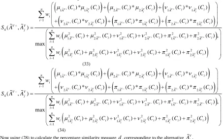
(3) Based on (22), we define the following:

1 1 2 2 1 1

1

2 2 1 1 2 2

4

2 2 2

1 2 1

(

) *

(

)

(

) *

(

)

(

) *

(

)

(

) *

(

)

(

) *

(

)

(

) *

(

)

(

,

)

(

)

(

)

(

max

V V V V V V

j j j

V V V V V V

j j j

V V V

n A i A i A i A i A i A i

i i

i i i i i i

A A A A A A

V V

j

i _A i _A i _A

C

C

C

C

C

C

w

C

C

C

C

C

C

S

A

A

w

C

C

C

₂2 ₁2 ₂2

1

2 2 2 2 2 2

1 2 1 2 1 2

1

)

(

)

(

)

(

) ,

(

)

(

)

(

)

(

)

(

)

(

)

V V V

V V V V V V

j j j j j j

n

i _A i _A i _A i

i n

i A i A i A i A i A i A i

i

C

C

C

w

C

C

C

C

C

C

(33)

1 1 2 2 1 1

1

2 2 1 1 2 2

4

2 2 2

1 2 1

(

) *

(

)

(

) *

(

)

(

) *

(

)

(

) *

(

)

(

) *

(

)

(

) *

(

)

(

,

)

(

)

(

)

(

max

V V V V V V

j j j

V V V V V V

j j j

V V V

n A i A i A i A i A i A i

i i

i i i i i i

A A A A A A

V V

j

i A i A i A

C

C

C

C

C

C

w

C

C

C

C

C

C

S

A

A

w

C

C

C

₂2 ₁2 ₂2

1

2 2 2 2 2 2

1 2 1 2 1 2

1

)

(

)

(

)

(

) ,

(

)

(

)

(

)

(

)

(

)

(

)

V V V

V V V V V V

j j j j j j

n

i A i A i A i

i n

i A i A i A i A i A i A i

i

C

C

C

w

C

C

C

C

C

C

(34)

Now using (28) to calculate the percentage similarity measure

d

_jcorresponding to the alternative

A

V_j

.

3.6 NUMERICAL EXAMPLE:

Similarity measure of interval valued vague set has been illustrated in the following numerical example. Suppose that a high technology company needs to hire an engineer. Now there are eight candidates

A

A A

₁

,

₂

,...,

A

₈ and six benefit criteria are considered:

(1) Personality (

C

₁)

(2) Past experience (

C

₂)

(3) Education level (

C

₃)

(4) Self-confidence (

C

₄)

(5) Emotional steadiness (

C

₅)

(6) Oral communication skill (

C

₆).

The weight vector of these criteria

C i

_i

(

1, 2..., 6)

is

_w

(0.12, 0.3, 0.07, 0.25, 0.06, 0.2).

T

Assuming that the characteristics of the alternatives

A j

j

(

1, 2, 3, 4, 5, 6, 7, 8)

are represented by interval valued

vague sets as follow in table 1

Table 1 Candidates

1 V

A

2

V

A

3

V

A

4

V

A

5

V

A

6

V

A

4

V

A

5

V

A

( )

w

V

A

A

V

Personality

1

C

C

₁

C

₁

C

₁

C

₁

C

₁

C

₁

C

₁

C

₁

C

₁

C

₁

1 1 V

(

)

j

A

C

_{0.2 0.3 0.6 0.4 0.8 0.3 0.5 0 0.12 0.8 0} 1

2AVj

(

)

C

0.25 0.35 0.7 0.45 0.9 0.35 0.6 0.2 0.12 0.9 0.2

1 1V

(

)

j

A

C

_{0.6 0 0.2 0.1 0.1 0.3 0.4 0.8 0.12 0 0.8} 1

2AVj

(

)

C

0.5 0 0.1 0 0.05 0.2 0.3 0.7 0.12 0 0.7

1 1 V

(

)

j

Volume 2, Issue 4, April 2013

Page 326

1 2 V

(

)

j

A

C

_{0.25 0.65 0.2 0.55 0.05 0.45 0.1 0.1 0.12 0.1 0.1}

Past

experience

C

2

C

2

C

2

C

2

C

2

C

2

C

2

C

2

C

2

C

2

C

2

2 1 V

(

)

j

A

C

_{0.5 0.3 0.7 0.1 0.2 0.4 0.6 0.5 0.3 0.7 0.1}

2

2AVj

(

C

)

0.53 0.4 0.8 0.3 0.4 0.5 0.65 0.6 0.3 0.8 0.3

2 1V

(

)

j

A

C

_{0.2 0.6 0.1 0.1 0.5 0.4 0.3 0.1 0.3 0.1 0.6}

2 2AVj

(

)

C

0.15 0.5 0 0 0.2 0.3 0.2 0.05 0.3 0 0.5

2 1 V

(

)

j

A

C

_{0.3 0.1 0.2 0.8 0.3 0.2 0.1 0.4 0.3 0.2 0.3}

2 2AVj

(

)

C

0.32 0.1 0.2 0.7 0.4 0.2 0.15 0.35 0.3 0.2 0.2

Education

level

C

3

C

3

C

3

C

3

C

3

C

3

C

3

C

3

C

3

C

3

C

3

3 1AVj

(

)

C

0.1 0.5 0.5 0.5 0.4 0.2 0.3 0.3 0.07 0.5 0.1

3 2 V

(

)

j

A

C

_{0.2 0.6 0.55 0.6 0.45 0.3 0.35 0.4 0.07 0.6 0.2} 3

1AVj

(

)

C

0.4 0.1 0.4 0.2 0.4 0.6 0.3 0.4 0.07 0.1 0.6

3 2 V

(

)

j

A

C

_{0.3 0.05 0.3 0.1 0.3 0.5 0.2 0.3 0.07 0.05 0.5} 3

1AVj

(

)

C

0.5 0.4 0.1 0.3 0.2 0.2 0.4 0.3 0.07 0.4 0.3

3 2 V

(

)

j

A

C

_{0.5 0.35 0.15 0.3 0.25 0.2 0.45 0.3 0.07 0.35 0.3}

Self-confidence

C

4

C

4

C

4

C

4

C

4

C

4

C

4

C

4

C

4

C

4

C

4

4 1 V

(

)

j

A

C

_{0.2 0.3 0.1 0.5 0.6 0.2 0.4 0.7 0.25 0.7 0.1} 4

2 V

(

)

j

A

C

_{0.4 0.5 0.25 0.55 0.65 0.3 0.5 0.75 0.25 0.75 0.25} 4

1V

(

)

j

A

C

_{0.05 0.3 0.6 0.4 0.3 0.6 0.1 0.2 0.25 0.05 0.6} 4

2 V

(

)

j

A

C

_{0 0.2 0.5 0.3 0.2 0.5 0.05 0.1 0.25 0 0.5} 4

1 V

(

)

j

A

C

_{0.75 0.4 0.3 0.1 0.1 0.2 0.5 0.1 0.25 0.25 0.3} 4

2 V

(

)

j

A

C

_{0.6 0.3 0.25 0.15 0.15 0.2 0.45 0.15 0.25 0.25 0.25}

Emotional

steadiness

C

5

C

5

C

5

C

5

C

5

C

5

C

5

C

5

C

5

C

5

C

5

5 1AVj

(

)

C

0.5 0.2 0.7 0.3 0.4 0.5 0.1 0 0.06 0.7 0

5 2 V

(

)

j

A

C

_{0.65 0.3 0.75 0.35 0.45 0.55 0.2 0.25 0.06 0.75 0.2} 5

1AVj

(

)

C

0.3 0.05 0.2 0.6 0.2 0.4 0.1 0.6 0.06 0.05 0.6

5 2 V

(

)

j

A

C

_{0.2 0.01 0.1 0.5 0.1 0.3 0.05 0.5 0.06 0 0.5} 5

1AVj

(

)

C

0.2 0.75 0.1 0.1 0.4 0.1 0.8 0.4 0.06 0.25 0.4

5 2 V

(

)

j

A

C

_{0.15 0.69 0.15 0.15 0.45 0.15 0.75 0.25 0.06 0.25 0.3}

Communi-

cation skill

C

6

C

6

C

6

C

6

C

6

C

6

C

6

C

6

C

6

C

6

C

6

6 1 V

(

)

j