A Unified Formulation and Fast Accelerated Proximal
Gradient Method for Classification
Naoki Ito naoki [email protected]
Department of Mathematical Informatics The University of Tokyo
7-3-1 Hongo, Bunkyo-ku, Tokyo, 113-8656, Japan
Akiko Takeda [email protected]
Department of Mathematical Analysis and Statistical Inference The Institute of Statistical Mathematics
10-3 Midori-cho, Tachikawa, Tokyo 190-8562 Japan
Kim-Chuan Toh [email protected]
Department of Mathematics National University of Singapore
Blk S17, 10 Lower Kent Ridge Road, Singapore 119076, Singapore
Editor:Moritz Hardt
Abstract
Binary classification is the problem of predicting the class a given sample belongs to. To achieve a good prediction performance, it is important to find a suitable model for a given dataset. However, it is often time consuming and impractical for practitioners to try various classification models because each model employs a different formulation and algorithm. The difficulty can be mitigated if we have a unified formulation and an efficient universal algorithmic framework for various classification models to expedite the comparison of performance of different models for a given dataset. In this paper, we present a unified formulation of various classification models (includingC-SVM, `2-SVM,
ν-SVM, MM-FDA, MM-MPM, logistic regression, distance weighted discrimination) and develop a general optimization algorithm based on an accelerated proximal gradient (APG) method for the formulation. We design various techniques such as backtracking line search and adaptive restarting strategy in order to speed up the practical convergence of our method. We also give a theoretical convergence guarantee for the proposed fast APG algorithm. Numerical experiments show that our algorithm is stable and highly competitive to specialized algorithms designed for specific models (e.g., sequential minimal optimization (SMO) for SVM).
Keywords: restarted accelerated proximal gradient method, binary classification, mini-mum norm problem, vector projection computation, support vector machine
1. Introduction
Binary classification is one of the most important problems in machine learning. Among the wide variety of binary classification models which have been proposed to date, the most popular ones include support vector machines (SVMs) (Cortes and Vapnik, 1995; Sch¨olkopf et al., 2000) and logistic regression (Cox, 1958). To achieve a good prediction performance,
c
it is often important for the user to find a suitable model for a given dataset. However, the task of finding a suitable model is often time consuming and tedious as different classification models generally employ different formulations and algorithms. Moreover, the user might have to change not only the optimization algorithms but also solvers/software in order to solve different models. The goal of this paper is to present a unified formulation for various classification models and also to design a fast universal algorithmic framework for solving different models. By doing so, one can simplify and speed up the process of finding the best classification model for a given dataset. We can also compare various classification methods in terms of computation time and prediction performance in the same platform.
In this paper, we first propose a unified classification model which can express vari-ous models including C-SVM (Cortes and Vapnik, 1995),ν-SVM (Sch¨olkopf et al., 2000), `2-SVM, logistic regression (Cox, 1958), MM-FDA, MM-MPM (Nath and Bhattacharyya,
2007), distance weighted discrimination (Marron et al., 2007). The unified model is first formulated as an unconstrained `2-regularized loss minimization problem, which is further
transformed into the problem of minimizing a convex objective function (quadratic func-tion, plus additional terms only for logistic regression) over a simple feasible region such as the intersection of a box and a hyperplane, truncated simplex, unit ball, and so on. Taking different loss functions (correspondingly different feasible regions in the transformed prob-lem) will lead to different classification models. For example, when the feasible region is given by the intersection of a box and a hyperplane, the unified formulation coincides with the well-known C-SVM or logistic regression, and when the region is given by a truncated simplex, the problem is the same as the ν-SVM.
It is commonly acknowledged that there is “no free lunch” in supervised learning in the sense that no single algorithm can outperform all other algorithms in all cases. Therefore, there can be no single “best” software for binary classification. However, by taking ad-vantage of the above-mentioned unified formulation, we can design an efficient algorithm which is applicable to the various existing models mentioned in the last paragraph. Our proposed algorithm is based on the accelerated proximal gradient (APG) method (Beck and Teboulle, 2009; Nesterov, 2005) and during the algorithm, only the procedure for computing the projection onto the associated feasible region differs for different models. In other words, by changing the computation of the projection, our algorithm can be applied to arbitrary classification models (i.e., arbitrary feasible region) without changing the optimization algo-rithmic framework. The great advantage of our algorithm is that most existing models have simple feasible regions, which make the computation of the projection easy and efficient.
of our FAPG algorithm, though we can no longer ensure its theoretical convergence. To summarize, while our method has extensive generality, numerical experiments show that it performs stably and is highly competitive to specialized algorithms designed for specific classification models. Indeed, our method solved SVMs with a linear kernel substantially faster than LIBSVM (Chang and Lin, 2011) which implemented the SMO (Platt, 1998) and SeDuMi (Sturm, 1999) which implemented an interior-point method. Moreover, our FAPG method often run faster than the highly optimized LIBLINEAR (Fan et al., 2008) especially for large-scale datasets with feature dimensionn >2000. The FAPG method can be applied not only to the unified classification model but also to the general convex com-posite optimization problem such as `1-regularized classification models, which are solved
faster than LIBLINEAR in most cases. It may be better to think of a stochastic variant of our method for further improvement and we leave it as a future research topic. We focus here on the deterministic one as the first trial to provide an efficient unified algorithm which is applicable to all well-known existing classification models.
The rest of this paper is organized as follows. Section 2 introduces some preliminary definitions and results on binary classification models and the APG method. Section 3 presents a unified formulation of binary classification models. In Section 4, we provide solution methods for the unified formulation. We develop efficient algorithms for comput-ing projections which are used in the APG method. Then we design our FAPG method combined with various techniques to speed-up its practical convergence. The iteration com-plexity ofO (logk/k)2
of our algorithm is also established, wherekis the iteration counter. Numerical experiments are presented in Section 5.
2. Preliminaries
In this section, we introduce some preliminary definitions on binary classification models and the APG method.
2.1 Binary Classification Models
Let X ⊂ Rn be the input domain and {+1,−1} be the set of the binary labels. Suppose
that we have samples,
(x1, y1), . . . ,(xm, ym)∈ X × {+1,−1}.
Define M := {1, . . . , m}, M+ := {i ∈M |yi = +1}, and M− := {i ∈M |yi =−1}. Let
m+ =|M+|and m−=|M−|.
We compute (w, b) for a decision functionh(x) =w>x−busing these samples and use h(x) to predict the label for a new input point ˆx∈ X. If h( ˆx) is positive (resp. negative), then the label of ˆxis predicted to be +1 (resp. −1). Here we focus on linear learning models by using linear functions h(x), but the discussions in this paper can be directly applied to non-linear kernel models (Sch¨olkopf and Smola, 2002) using nonlinear maps φ(x) mapping
xfrom the original space to a high dimensional space.
and Bhattacharyya, 2007), the model based on Fisher’s discriminant analysis (MM-FDA) (Bhattacharyya, 2004; Takeda et al., 2013), and the logistic regression (Cox, 1958).
Many binary classification models have the following formulation which consists of the sum of loss of each sample and a regularization term:
min
w,b m
X
i=1
` yi(w>xi−b)
+ 1 Ckwk
p
p, (1)
where `:R→R is a proper, closed, and convex function; C >0 is a parameter; and k·kp is the p-norm withp∈[1,∞].
2.2 Accelerated Proximal Gradient Method
In this section, we first introduce the accelerated proximal gradient (APG) method (Beck and Teboulle, 2009) which is designed for the following problem:
min
α∈Rd
F(α) :=f(α) +g(α). (2)
Note that one can express a minimization problem constrained over a set S in the form of (2) by setting g=δS, where
δS(α) =
(
0 (α∈S) +∞ (α6∈S)
is the indicator function of the setS.
To apply the APG method to (2), we need to assume the following conditions:
1. g : Rd → R ∪ {+∞} is a proper, closed, and convex function which is possibly
nonsmooth. Its effective domain dom(g) = {α ∈ Rd | g(α) < +∞} is closed and
convex.
2. f :Rd→R is a proper, closed, convex, and continuously differentiable function, and
its gradient ∇f(·) is Lipschitz continuous on Rd,1 i.e., there exists a constant L > 0
such that
k∇f(α)− ∇f(β)k2 ≤Lkα−βk2 ∀α,β∈Rd. (3)
The minimum value of such Lis referred to as the Lipschitz constantLf of ∇f(·).
3. The problem (2) is solvable, i.e., the optimal value is finite and an optimal solution
α∗ exists.
Let L≥Lf. We define an approximate functionQL:Rd→ Rof f(α) around β and a
mappingTL(α) :Rd→Rd as follows:
QL(α;β) =f(β) +h∇f(β),α−βi+
L
2kα−βk
2
2+g(α)
TL(β) = argmin
α∈Rd
QL(α;β).
1. It is sufficient if∇f(·) is Lipschitz continuous on a neighborhood of dom(g): the convex hull of dom(g)∪ {βk|
The basic proximal gradient (PG) method generates a sequence{αk}∞
k=0 by αk+1 =TL(αk) = argmin
α∈Rd n
g(α) +L 2
α−
αk− 1 L∇f(α
k) 2 2 o
= proxg,Lαk− 1 L∇f(α
k),
where proxg,L( ¯α) := argminα∈Rd n
g(α) +L
2kα−α¯k 2 2 o
is the proximal operator ofg. Ifg= δS, then proxg,Lk =PS, wherePS( ¯α) = argminα∈Skα−α¯k2 is the orthogonal projection of
¯
αonto the setS. In this case, the above PG method coincides with the gradient projection method. If g(·) = k · k1, then proxg,L(α)
i = sign(αi) max{0,|αi| −L} (i = 1,2, . . . , d) which is known as the soft-thresholding operator. Other analytical computations of the proximal operators of variousg can be found in (Parikh and Boyd, 2014, Section 6).
It is known that the PG method has the iteration complexity such thatF(αk)−F(α∗)≤
O(1/k), where α∗ is an optimal solution of (2). The APG method (Beck and Teboulle,
2009), which is also known as FISTA, is an acceleration of the PG method. It generates two sequences
βk ∞ k=1 and
αk ∞
k=0. For an arbitrary initial point β
1 = α0 ∈
Rd and
t1 = 1, the APG method solves (2) through the following steps (k= 1,2, . . .):
Accelerated Proximal Gradient Method
Step 1. Compute
αk=TL(βk) = proxg,L
βk− 1
L∇f(β
k).
Step 2. Compute tk+1=
1+√1+4t2
k
2 .
Step 3. Compute βk+1 =αk+tk−1
tk+1(α
k−αk−1).
For the APG method, the iteration complexity result such that F(αk)−F(α∗)≤O(1/k2)
is known (see (Beck and Teboulle, 2009, Theorem 4.4)). The second term ttk−1
k+1(α
k−αk−1)
in Step 3 can be seen as the momentum of the sequence {αk}∞
k=0. It enlarges the moving
distance of the sequences {α}∞
k=0,{β} ∞
k=1 which may lead them closer to the optimumα ∗
more quickly. While various other APG methods (e.g, (Nesterov, 2013; Monteiro et al., 2016; Su et al., 2014)) are proposed, the above APG (namely, FISTA) is used in many applications because it is simpler to implement.
It is known that α∗ is an optimal solution of (2) if and only if α∗ = TL(α∗). More specifically, the necessary and sufficient optimality condition forα∗to be an optimal solution
of (2) is
∃γα∈∂g(α∗) s.t. h∇f(α∗) +γα, α−α∗i ≥0, ∀α∈Rd. (4)
On the other hand, from the definition of TL(β), we have
∃γβ ∈∂g(TL(β)) s.t. h∇f(TL(β))+L TL(β)−β
+γβ, α−TL(β)i ≥0, ∀α∈Rd, (5)
for anyβ∈Rd. The termL TL(β)−β
in (5) can be seen as the residual of the optimality condition (4). Thus it would be a natural criterion to terminate the APG if LkTL(αk)−
αkk
Despite having a strong iteration complexity result, the APG method may still not be efficient enough for practical purpose. In the following, we describe several well-known strategies to make the APG method practically efficient.
2.2.1 Backtracking Strategy
We assume thatLis greater than or equals to the Lipschitz constantLf of∇f(α). However it is advantageous to use a smaller value forLwhenever possible since the constantLplays the role of a step size as in a gradient descent method; fixingLto be the Lipschitz constant Lf is usually too conservative (see Table 5 in Section 5). Thus we adopt the following backtracking strategy (Beck and Teboulle, 2009) after Step 1 with arbitrary given constants ηu >1 andL0>0:
‘bt’: While
F(αk)> Q Lk(α
k;βk), (6)
updateLk←ηuLk andαk←TLk(β
k). Set L
k+1←Lk.
The inequality (6) in ‘bt’ ensures that the complexity resultF(αk)−F(α∗)≤O(1/k2) still
holds. We note that the inequalityF(αk)≤Q Lk(α
k;βk) is satisfied ifL
k≥Lf, i.e., it is a weaker condition than (3).
2.2.2 Decreasing Strategy for Lk
Beck and Teboulle (2009) designed the backtracking strategy ‘bt’ so that the values of Lk is non-decreasing. In fact, the convergence analysis of (Beck and Teboulle, 2009) requires the value ofLk to be non-decreasing. However, it is advantageous to decrease the value of
Lk whenever possible since the constant L1k gives a larger step size.
To allow Lk to decrease, Scheinberg et al. (2014) modifies the APG method so that {tk}∞k=1 satisfies tk/Lk ≥ tk+1(tk+1 −1)/Lk+1 (∀k ≥ 1) and the sequences {αk}∞k=0 and
{βk}∞
k=1 are generated along with {tk}∞k=1. To be specific, let us introduce the following
simple step to decrease the value ofLk, where ηd>1 is a given constant.
‘dec’: SetLk+1←Lk/ηd.
The modified APG of (Scheinberg et al., 2014) can be described as in Algorithm 1. It differs from the original APG in that the updates of tk and βk are added to ‘bt’ and Step 2 is modified. The convergence of Algorithm 1 is shown as follows.
Proposition 1 (from Scheinberg et al., 2014) LetS∗ be the set of optimal solutions of
(2). For anyα∗ ∈S∗, the sequence{αk}∞
k=0generated by Algorithm 1 satisfies the following
inequality:
F(αk)−F(α∗)≤ 2ηuLfkα
0−α∗k2 2
Algorithm 1An Accelerated Proximal Gradient Method with Non-Monotonic Backtrack-ing
Input: f,∇f,g, proxg,L, >0,L1 =L0 >0,ηu>1,ηd>1,kmax>0, β1 =α0 Output: αk
Initialize: t1 ←1, t0←0
for k= 1, . . . , kmax do
αk←T Lk(β
k) = prox g,Lk
βk− 1
Lk∇f(β
k) # Step 1
whileF(αk)> Q Lk(α
k;βk) do
Lk←ηuLk # ‘bt’
tk←
1+q1+4(Lk/Lk−1)t2k−1
2 βk ←αk−1+tk−1−1
tk (α
k−1−αk−2) αk←T
Lk(β
k) = prox g,Lk
βk− 1
Lk∇f(β
k)
end while if kLk(TLk(α
k)−αk)k< then
break end if
Lk+1←Lk/ηd # ‘dec’
tk+1←
1+√1+4(Lk+1/Lk)t2k
2 # Step 2’
βk+1 ←αk+tk−1
tk+1(α
k−αk−1) # Step 3
end for
2.2.3 Restarting Strategy
The value tk−1
tk+1 ∈[0,1) in Step 3 determines the amount ofmomentumin tk−1
tk+1(α
k−αk−1).
When the value tk−1
tk+1 is close to 1, i.e., the momentum is high, the sequences of solutions {αk}∞
k=0 and {βk}∞k=1 would overshoot and oscillate around the optimal solution α∗. In
order to avoid the oscillation and further speed up the convergence, O’Donoghue and Cand`es (2015) introduced an adaptive restarting strategy:
‘re’: If ∇f(βk)>(αk−αk−1) +g(αk)−g(αk−1)>0,
then updatetk+1 ←1, tk←0,βk+1 ←αk−1, and αk←αk−1.
Roughly, the APG method resets the momentum back to zero and restarts from the previous pointαk−1if the direction of motionαk−αk−1seems to cause the (approximated) objective
value to increase, which may be a sign of overshooting. Note that the computational cost of ‘re’ is inexpensive since∇f(βk) has already been computed at Step 1. O’Donoghue and Cand`es (2015) also provided a heuristic convergence analysis for their restarting scheme (‘re’) when f is a strongly convex (i.e., there exists a constant µ > 0 such that f(α)−
µ
2kα−α ∗k2
2 is convex) quadratic function andg = 0. However, the convergence of ‘re’ for
a general strongly convex objective function is unknown (not to mention for the general non-strongly convex function in our problem).
k
iter
0
K1
K2
K3
restart
restart
restart
¯
k1
¯
k2
¯
k
3Figure 1: Illustration of Maintaining Top-Speed Strategy (‘mt’). A prohibition period of restart forKi iteration are imposed after thei-th restart occurs. If the condition ∇f(βk)>(αk−αk−1) < 0 is satisfied after the period passed, then the (i+
1)-th restart occurs. The next prohibition period is doubled, i.e., Ki+1 = 2Ki. ¯
ki(≥Ki) denotes the number of iteration taken between the (i−1)-th andi-th restart, which will be used to convergence analysis in Section 4.2.
Nesterov (2013) proposed a restarting method, which has asymptotic linear convergence if g is strongly convex. Lin and Xiao (2015) showed that a similar restart technique can achieve the same convergence rate as Nesterov’s scheme if f is strongly convex. Su et al. (2014) modeled the APG method as a second-order ordinary differential equation (ODE). They provided a speed restarting framework that ensures a linear convergence of the ODE with respect to time in the case that f is strongly convex and g = 0. To the best of our knowledge, none of the restarting schemes have convergence guarantees for a general non-strongly convex function.
2.2.4 Maintaining Top-Speed Strategy
The restarting strategy cancels out high momentum and prevents overshooting. In the neighborhood of an optimum, however, maintaining high momentum may be effective rather than restarting APG (see Figures 6 and 8 in Section 5), because large overshooting may not occur. Thus we put a prohibition period of restart forKi iteration after thei-th restart occurs, where Ki increases as Ki = 2Ki−1 (i = 2,3, . . .) and K1 ≥ 2. See Figure 1 for
illustration. Precisely, letting k = kre be the iteration count at which the last restart occurs, we introduce the following step:
‘mt’: If k≤kre+Ki, then skip ‘re’. If restart occurs, then updatekre ←k,Ki+1 ←2Ki, and i←i+ 1.
While a similar strategy is taken in the experiment of (Monteiro et al., 2016), its con-vergence analysis is not provided. One of our contributions in this paper is to show that in fact the modification ‘mt’ of the restarting strategy can ensure the convergence rate of O (logk/k)2
under a mild assumption. We will elaborate it in Section 4.2.
3. New Unified Formulation
In this paper, we focus on the following `2-regularized loss minimization problem:
min
w,b L(Ae
>w
−ab) + 1 2Ckwk
2
where L:Rm →R is a proper, closed, and convex function; Ae∈Rn×l,a ∈Rl, andC >0
is a parameter. We will later show examples such that
• l=m, Ae=Xe := [y1x1, y2x2, . . . , ymxm], a=y, and
• l=n, Ae=I, a=0.
Our algorithm to be described later can be applied to a more general loss-regularized model with p∈(1,∞):
min
w,b
L(Ae>w−ab)| kwkp≤λ , (8)
where λ > 0 is a parameter. We note that the condition p ∈ (1,∞) is required for our unified classification algorithm because the smoothness of the dual norm ofk · kp is required to apply the APG method to the dual problem of (8). However, if p ∈ {1,∞} and L is smooth, the APG method can be applied to the primal problem (8). See Appendix D for `1-regularized problems, i.e., the case ofp= 1.
3.1 Dual Formulation
The dual problems of (7) is given by
min
α n
L∗(−α) +C 2kAeαk
2
2|α>a= 0 o
, (9)
whereL∗(α) = sup
z{α>z− L(z)} is the convex conjugate ofL.
The dual problem of (8) is
min
α
L∗(−α) +λkAeαk∗p |α>a= 0 , (10)
where kzk∗
p = supkwkp≤1{z>w} is the dual norm ofk · kp. It is known that k · k∗p =k · kq, where q = p/(p−1). The problem (10) can be seen as the Fenchel dual of (8), whose derivation is shown in Appendix A. We note that the norms k · kp and k · k∗q are smooth for
p∈(1,∞).
As shown later, in all classification models, L∗ is the sum of a smooth function and an
indicator function of a simple setS for which the projectionPScan be computed efficiently. Thus we can apply the APG method as an acceleration of the gradient projection method to the dual problems (9) and (10). By this construction, we can ensure the fast convergence rate of F(αk)−F(α∗) ≤ O(1/k2) for various classification models in a unified way. In
other word, the APG method can obtain a solution with desired accuracy >0 inO(1/√) iteration.
There is an existing work (Zhou et al., 2010) which applies the APG method to the primalC-SVM, i.e., (7) with the hinge loss function. However, their method requiresO(1/) iteration to obtain a solution with the desired accuracy >0 because it approximates the hinge loss by a smoothed function and making the approximation tighter requires extra iterations (Nesterov, 2005).
3.2 Relation to Existing Binary Classification Models
3.2.1 C-SVM
Let Ae = Xe and a = y in (7). Let `(z) = max{0,1−z} be the hinge loss and L(z) = Pm
i=1`(zi). Then the primal problem (7) is known as the standard C-SVM (Cortes and
Vapnik, 1995). Since
L∗(−α) = m
X
i=1
`∗(−αi), where `∗(−α) =
(
−α ifα∈[0,1] +∞ otherwise,
the dual problem (9) can be reduced to
min
α
C 2kXeαk
2 2−α
>
e+δSC(α), (11)
whereSC ={α∈Rm |α>y= 0, 0≤α≤e}.
3.2.2 `2-SVM
Let Ae= Xe and a = y in (7). Let `(z) = (max{0,1−z})2 be the truncated squared loss
and L(z) =Pm
i=1`(zi). Then the primal problem (7) is known as the`2-SVM. Since
L∗(−α) = m
X
i=1
`∗(−αi), where `∗(−α) =
(α2
4 ifα≥0
+∞ otherwise,
the dual problem (9) can be reduced to
min
α
C 2kXeαk
2 2+k
αk2 2
4 +δS`2(α), (12)
whereS`2 ={α∈R
m|α>y= 0, α≥0}.
3.2.3 Logistic regression
Let Ae = Xe and a = y in (7). Let `(z) = log(1 + exp(−z)) be the logistic loss and
L(z) = Pm
i=1`(zi). Then the primal problem (7) is the logistic regression (Cox, 1958).
Since
L∗(−α) = m
X
i=1
`∗(−αi), where `∗(−α) =
αlog(α) + (1−α) log(1−α) (0< α <1)
0 (α= 0,1)
+∞ otherwise,
the dual problem (9) can be reduced to
min
α
C 2kXeαk
2 2+
X
i:αi>0
αilog(αi) +
X
i:αi<1
(1−αi) log(1−αi) +δSLR(α), (13)
whereSLR ={α∈Rm|α>y= 0, 0≤α≤e}.
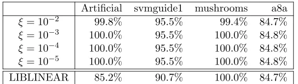
its optimal solution α∗ satisfies0<α∗ <e (Yu et al., 2011), we can instead solve (13) by
replacing SLR by SLR(ξ) := {α ∈ Rm | α>y = 0, ξe ≤ α ≤ (1−ξ)e}, where ξ > 0 is a
small constant. The second and third terms in (13) are differentiable over SLR(ξ). We will
later show numerically that the resulting decision hyperplane is robust to a small deviation of ξ (see Table 6 in Section 5).
3.2.4 ν-SVM
LetAe=Xe and a=yin (7). Let
L(z) = min ρ
n
−ρ+ 1
mν
m
X
i=1
max{ρ−zi,0}
o
,
where ν ∈(0,1] is a given parameter. The function L(z), known as the conditional value-at-risk (CVaR) (Rockafellar and Uryasev, 2000), is the expected value of the upper ν-tail distribution. Gotoh and Takeda (2005) pointed out that minimizing CVaR is equivalent to ν-SVM (Sch¨olkopf et al., 2000), which is also known to be equivalent toC-SVM.
Since
L∗(−α) =
(
0 e>α= 1 and α∈h0,mν1 im +∞ otherwise,
the dual problem is given by
min
α
C 2kXeαk
2
2+δSν(α), (14)
where Sν = {α ∈ Rm | α>y = 0, α>e = 1, 0 ≤ α ≤ mν1 e} is the intersection of the
hyperplane{α|α>y= 0}and the truncated simplex {α|α>e= 1, 0≤α≤ 1
mνe}. Note that any positive value forC does not change the optimal solution of (14), and therefore, we can set C = 1. There exists a valid range (νmin, νmax]⊆(0,1] for ν, where νmin is the infimum of ν >0 such that Xeα∗ 6=0, andνmax :=
2 max{m+,m−}
m is the maximum ofν ≤1 for which Sν 6= φ. Since the parameter ν takes a value in the finite range (νmin, νmax], choosing the parameter value forν-SVM is often easier than that for C-SVM.
3.2.5 Distance Weighted Discrimination (DWD)
Let Ae = Xe, a = y, λ = 1 and p = 2 in (8). For a positive parameter ν, let `(z) be the
function defined by
`(z) = min ρ
n1
ρ + 1
mν(ρ−z)|ρ≥z, ρ≥ √
mνo
=
(1
z ifz≥
√ mν
2√mν−z
mν otherwise
.
ConsiderL(z) =Pm
i=1`(zi).This loss function is used in the distance weighted
have
L∗(−α) = m
X
i=1
`∗(−αi), where `∗(−α) =
(
−2√α 0≤α≤ 1
mν
+∞ otherwise,
the dual problem (9) can be equivalently reduced to
min
α n
kXeαk2−2
m
X
i=1
√
αi+δSDWD(α)
o
, (15)
whereSDWD =
α∈Rm|α>y= 0, 0≤α≤ mν1 e .
As in the case of the logistic regression, the second term in (15) is not differentiable at αi = 0 (i∈M). However, since it is known that there exists an optimal solution α∗ such that α∗
i > 0 (i ∈ M), we can solve (15) by replacing SDWD by SDWD(ξ) =
α ∈ Rm |
α>y = 0, ξe ≤ α ≤ 1
mνe where ξ > 0 is a small constant. The second term in (15) is differentiable overSDWD(ξ).
3.2.6 Extended Fisher’s discriminant analysis (MM-FDA)
The well-known Fisher’s discriminant analysis (FDA) uses a decision function to maximize the ratio of the variance between the classes to the variance within the classes. Let ¯xo and Σo, o ∈ {+,−}, be the mean vectors and the positive definite covariance matrices of xi,
i∈Mo, respectively. Then FDA is formulated as follows:
max
w
w>( ¯x+−x¯−)2 w>(Σ
++ Σ−)w
.
Its optimal solution is given by
w∗ = (Σ++ Σ−)−1( ¯x+−x¯−).
LetAe=I anda=0in (7). Here we consider the mean-standard deviation type of risk
corresponding to FDA:
L(w) =−w>( ¯x+−x¯−) +κ q
w>(Σ
++ Σ−)w,
whereκ >0 is a parameter. Since
L∗(−α) = sup
w n
−α>w+w>( ¯x+−x¯−)−κ q
w>(Σ
++ Σ−)w o
= sup
w
min
kuk2≤κ
n
−α>w+w>( ¯x+−x¯−) +w>(Σ++ Σ−)1/2u o
= min
u
δSFDA(u)|α= ( ¯x+−x¯−) + (Σ++ Σ−)
1/2u ,
whereSFDA =
u∈Rn| kuk2 ≤κ , the dual problem (9) can be reduced to
min
α,u n
δSFDA(u) +
C 2kαk
2
2 |α= ( ¯x+−x¯−) + (Σ++ Σ−)1/2u o
which is equivalent to
min
u
δSFDA(u) +
( ¯x+−x¯−) + (Σ++ Σ−)1/2u 2
2 . (16)
Takeda et al. (2013) showed that
κmax:=
infu,κ κ s.t. minu
( ¯x+−x¯−) + (Σ++ Σ−)1/2u
2+δSFDA(u) = 0
is equivalent to FDA. Hence (16) can be seen as an extension of FDA. We will refer it as MM-FDA in this paper.
3.2.7 Maximum Margin Minimax Probability Machine (MM-MPM)
LetAe=I anda=0 in (7). We consider a class-wise mean-standard deviation type of risk:
L(w) =−w>x¯++κ q
w>Σ +w
−−w>x¯−+κ q
w>Σ −w
.
Similar to MM-FDA, we have
L∗(w) = sup
w n
−α>w+w>x¯+−κ q
w>Σ +w
−w>x¯−−κ q
w>Σ −w
o
= sup
w
min
ku+k2≤κ
ku−k2≤κ
n
−α>w+ w>x¯++w>Σ 1/2 + u+
− w>x¯−+w>Σ1−/2u− o
= min
u+,u−
δSMPM(u+,u−)|α= ¯x++ Σ
1/2 + u+
− x¯−+ Σ1−/2u− ,
where SMPM =
(u+,u−) ∈Rn×Rn | ku+k2 ≤ κ, ku−k2 ≤κ . Thus the dual problem
(9) can be reduced to
min
α,u+,u−
n
δSMPM(u+,u−) +
C 2kαk
2
2 |α= ¯x++ Σ1+/2u+
− x¯−+ Σ1−/2u− o
,
which is equivalent to
min
u+,u−
δSMPM(u+,u−) +
x¯++ Σ1+/2u+
− x¯−+ Σ1−/2u−
2
2 . (17)
The last problem (17) is equivalent to the dual of the maximum margin minimax probability machine (MM-MPM) (Nath and Bhattacharyya, 2007).
4. A Fast APG method for Unified Binary Classification
4.1 Vector Projection Computation
When applying the APG method to a constrained optimization problem over S, the pro-jectionPS ontoS appears at Step 1. We need to change the computation of the projection
PS depending on the definition ofS. In this section, we provide efficient projection compu-tations for SC,S`2,SLR(ξ),Sν,SDWD(ξ), SMPM, and SFDA.
4.1.1 Bisection Method for Projection
Many models shown in Section 3 have a linear equality and box constraints. Here we consider the set S ={α ∈ Rm | α>e= r, l ≤αi ≤u (∀i ∈M)} and provide an efficient algorithm for computing the projection PS(α¯):
min
α n1
2kα−α¯k
2
2 |α>e=r, l≤αi≤u, (i∈M)
o
. (18)
We assume that (18) is feasible. One way to solve (18) is to use breakpoint search algorithms (e.g., (Helgason et al., 1980; Kiwiel, 2008; Duchi et al., 2008)). They are exact algorithms and have linear time complexity ofO(m). Helgason et al. (1980); Kiwiel (2008) developed the breakpoint search algorithms for the continuous quadratic knapsack problem (CQKP) which involves the projection (18) as a special case. By integrating the breakpoint search algorithm and the red-black tree data structure, Duchi et al. (2008) developed an efficient update algorithm of the gradient projection method when the gradient is sparse.
In this paper, we provide a numerical algorithm for (18). Although its worst case complexity is Omlog α¯max−¯αmin
0
, where ¯αmax= max{α¯i |i∈M} and ¯αmin = min{α¯i |
i∈M}, it often requires less time to compute a solution ˆαsuch thatkαˆ−PS(α¯)k∞< 0=
uin practice, whereu≈2.22×10⁻¹⁶is the IEEE 754 double precision. Note that the error
ucan occur even when using the breakpoint search algorithm becauseuis the supremum of the relative error due to rounding in the floating point number system. Thus, it is sufficient to choose 0=uas the stopping tolerance for our algorithm in practice. 2
The difference between the algorithms is that the breakpoint search algorithms use binary search, whereas our algorithm uses bisection to solve an equation. It is known that the projection (18) can be reduced to finding the root of an one dimensional monotone function.
Lemma 2 (e.g. Helgason et al., 1980) Suppose that the problem (18) is feasible. Let
αi(θ) = min
n
max{l,α¯i−θ}, u
o
, i∈M
and let
h(θ) =X i∈M
αi(θ).
The following statements hold:
2. Another practical way is to decrease0, i.e., to improve the accuracy of the projection progressively, as APG iterates. The APG method with the inexact computation also share the same iteration complexity
−1 −0.5 0 0.5 1 0
0.5 1 1.5 2
θ
h
Figure 2: Illustration of the function h(θ) := P
i∈Mαi(θ). The function h is piecewise linear.
1. h(θ) is a continuous, non-increasing, and piecewise linear function which has break-points at α¯i−u and α¯i−l (i∈M).
2. There exists θ∗ ∈(¯α
min− mr,α¯max−mr) such thath(θ∗) =r.
3. Let αˆi=αi(θ∗), i∈M. Then αˆ is an optimal solution of (18).
An example ofh(θ) is illustrated in Figure 2. To solveh(θ) =r, the breakpoint search uses the binary search to find two adjacent breakpoints that contain a solutionθ∗ between them. Then the exact solutionθ∗ can be obtained by linear interpolation of the two breakpoints.
Instead of binary search, we employ the bisection method to solve the equationh(θ) =r.
Bisection Algorithm for Projection
Step 1. Setθu= ¯α
max−mr andθl= ¯αmin−mr.
Step 2. Set ˆθ= (θu+θl)/2
Step 3. Compute h(ˆθ).
Step 4. If h(ˆθ) =r, then terminate with ˆθ∗= ˆθ. Else if h(ˆθ)< r, then set θu= ˆθ.
Else if h(ˆθ)> r, then set θl= ˆθ.
Step 5. If |θu−θl|< 0, then terminate with ˆθ∗= ˆθ. Else, go to Step 2.
All steps require at mostO(m) operations and the maximum number of iteration is
log(α¯max−¯αmin
0 )
. Thus, the computational complexity of the bisection algorithm is at mostO mlog(α¯max−¯αmin
0 )
. As the bisection method narrows the interval (θl, θu), some of the terms α
for given θl and θu satisfyingθl< θu:
U :={i∈M |α¯i−θu ≥u (i.e.,αi(θ) =u, ∀θ∈[θl, θu])}
L :={i∈M |α¯i−θl≤l (i.e.,αi(θ) =l, ∀θ∈[θl, θu])}
I :=M\(U ∪L).
If ¯αi−θu ≥l and ¯αi−θl≤u∀i∈I, then
θ=|U|u+|L|l+X i∈I
αi−r
/|I| (19)
is an exact solution. IfI 6=φ, then we also divideI into the following three disjoint sets for given ˆθ∈(θl, θu):
IU ={i∈I |α¯
i−θˆ≥u, (i.e.,αi(θ) =u ∀θ∈[θl,θˆ])}
IL ={i∈I |α¯
i−θˆ≤l, (i.e.,αi(θ) =l ∀θ∈[ˆθ, θu])}
IC =I\(IU ∪IL)
Then we have
h(ˆθ) = X i∈M
αi(ˆθ) =|U|u
| {z }
su
+|IU|u
| {z } ∆su
+|L|l
|{z}
sl
+|IL|l
| {z } ∆sl
+X
i∈IC
αi
| {z }
sc
−|IC|θ.ˆ
By storing the value of each terms, we can reduce the number of additions. The resulting algorithm can be described as Algorithm 2.
Compared to the existing breakpoint search algorithms, our bisection method can avoid the computation of breakpoints and the comparison between them. In many cases, our algorithm can obtain the exact solution by (19). It is often faster than the breakpoint search algorithms in practice (see Table 2 in Section 5).
Remark 3 Mimicking (Kiwiel, 2008), we can divide the set M more finely and reduce the recalculation of certain sums as shown in Appendix B. However, Algorithm 2 allows for simpler implementation and runs faster on our computer systems.
In the followings, we use Algorithm 2 to compute the projection ontoSC, S`2, SLR(ξ), SDWD(ξ) and Sν.
4.1.2 Projection for C-SVM, Logistic Regression, `2-SVM, DWD
The projection for C-SVM, logistic regression, `2-SVM, and DWD can be formulated as
follows:
min
α n1
2kα−α¯k
2 2 |y
>
α= 0, l≤αi≤u (i∈M)
o
, (20)
where (l, u) = (0,1) for C-SVM, (l, u) = (0,∞) for `2-SVM, (l, u) = (ξ,1−ξ) for logistic
regression, and (l, u) = ξ, 1
mν
for DWD. By transforming the variableα and the vectorα¯ to
βi =
(
αi ifyi= 1
−αi+l+u otherwise
and β¯i =
(
¯
αi ifyi = 1
Algorithm 2 Bisection Algorithm for (18) INPUT: α¯, r, l, u, 0>0 OUTPUT:α
INITIALIZE: I ←M, su←sl←sc←0, θu←α¯max−mr, θl←α¯min−mr # Step 1
while |θu−θl|> 0 do
ˆ
θ← θu+θl
2 # Step 2
ˆ
u←u+ ˆθ, ˆl←l+ ˆθ IU ← {i∈I |α¯
i≥uˆ}, IL← {i∈I |α¯i≤ˆl} # Step 3
IC ←I\(IU∪IL)
∆su ← |IU|u, ∆sl ← |IL|l, sc←Pi∈ICαi
val←su+ ∆su+sl+ ∆sl+sc− |IC|θˆ
if val < rthen # Step 4
θu ←θˆ, I ←IC ∪IL
su←su+ ∆su
else if val > r then θl←θˆ, I ←IC∪IU
sl←sl+ ∆sl
else break end if
if α¯i−θu≥land ¯αi−θl≤u ∀i∈I then ˆ
θ←(su+sl+sc−r)/|I|
break end if end while
respectively, the problem (20) can be reduced to
min
β n1
2kβ−β¯k
2
2 |e>β= (l+u)m−, l≤βi≤u (i∈M)
o
.
The last problem can be solved by Algorithm 2.
4.1.3 Projection for ν-SVM
In applying the APG method toν-SVM, we shall be concerned with the projectionPSν(α¯):
min
α n1
2kα−α¯k
2 2
α>y= 0, α>e= 1, 0≤α≤
1 mνe
o
. (21)
Letα+ and α− be the subvectors ofα corresponding to the label +1 and−1, respectively.
Lete+ ande− be subvectors ofewith sizem+ andm−. From the fact that the conditions α>y= 0 and α>e= 1 are equivalent toα>oeo = 12 (o∈ {+,−}), the problem (21) can be decomposed into the following two problems:
min
αo n1
2kαo−α¯ok
2 2
e>oα=
1
2, 0≤αo ≤ 1 mνeo
o
, o∈ {+,−}. (22)
Then, Algorithm 2 can be applied to solve (22).
4.1.4 Projection for MM-MPM and MM-FDA
The projection PSFDA( ¯α) of ¯α onto SFDA=
α∈Rn| kαk2 ≤κ is easy to compute; We
have
PSFDA( ¯α) = min
n
1, κ kα¯k2
o
¯
α.
Similarly, the projection PSMPM(α¯+,α¯−) for MM-MPM can be computed as follows:
PSMPM( ¯α+,α¯−) =
minn1, κ kα¯+k2
o
¯
α+,min n
1, κ kα¯−k2
o
¯
α−
.
4.2 Convergence Analysis of a Fast APG Method with Speed-up Strategies
We have shown several strategies to speed-up the APG method in Section 2. While the convergence proof has been shown for the backtracking ‘bt’ and decreasing ‘dec’ strategy, the convergence for the restart ‘re’ and maintaining top-speed ‘mt’ strategy is unknown. In this section, we develop a fast APG (FAPG) method by combining all these techniques and show its convergence.
4.2.1 A Fast APG with Stabilization
In addition to the techniques in Section 2, we also employ the following practical stabilization strategy, where it doesnot affect our convergence analysis.
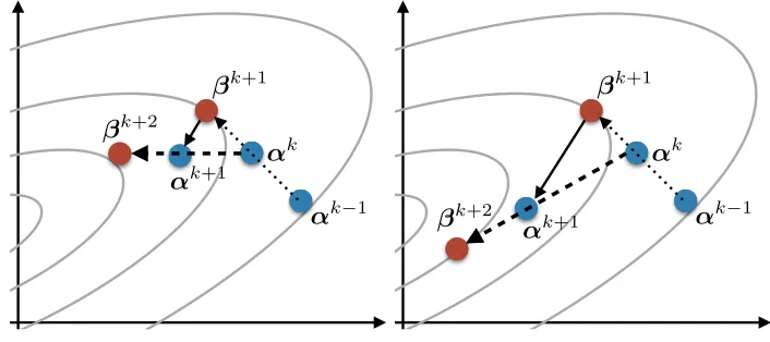
ç
k+1
↵k ↵k+1
↵k 1 k+2
ç
k+1
↵k 1 ↵k
↵k+1 k+2
Figure 3: Effects of the value of Lk to the momentum ttkk−1+1(αk−αk−1) (left: Lk is large, right: Lk is small). A smaller value of Lk gives a larger step size at Step 1 as illustrated by the solid lines. This results in high momentum at Step 3 as illustrated by the dashed lines.
This inherently induces high momentum (as illustrated in Figure 3). On the other hand, the restarting strategy cancels out high momentum. Hence combining them triggers the restart frequently and makes the APG method unstable. In order to avoid the instability, it would be necessary to reduce theηd (rate of decreasingLk) near the optimum. The restart would occur when the sequences approach the optimum. Therefore we take the following strategy to reduce the value ofηd with a constant δ∈(0,1):
‘st’: Updateηd←δ·ηd+ (1−δ)·1 when the restart occurs.
Algorithm 3 is our FAPG method which combines these strategies. The difference from Algorithm 1 is the “if block” after Step 3.
4.2.2 Convergence Analysis
Let ¯ki denotes the number of iteration taken between the (i−1)-th and the i-th restart (see Figure 1 for illustration). In the followings, we denoteαkasα(j,kj+1) ifk=Pj
i=1¯ki+
kj+1 (¯kj+1 ≥ kj+1 ≥ 0). In other word, α(i,ki+1) denotes a point obtained at the ki+1-th
iteration counting from the i-th restart. Note that α(i+1,0) =α(i,k¯i+1−1) (∀i≥0). We will frequently switch the notations αk andα(i,ki+1) for notational convenience.
The following lemma is useful to evaluate the function F.
Lemma 4 (from Beck and Teboulle, 2009) If F(TL(β))≤QL(TL(β);β), then
F(TL(β))−F(α)≤
L 2
kβ−αk2
2− kTL(β)−αk22 , ∀α∈Rd.
Algorithm 3 A Fast Accelerated Proximal Gradient (FAPG) Method with Speeding-Up Strategies
Input: f,∇f,g, proxg,L, >0,L1=L0>0,ηu >1,ηd>1,kmax >0,β1=α0 =α−1,
K1 ≥2,δ ∈(0,1)
Output: αk
Initialize: t1 ←1, t0←0, i←1, kre←0
for k= 1, . . . , kmax do
αk←T Lk(β
k) = prox g,Lk
βk− 1
Lk∇f(β
k) # Step 1
whileF(αk)> Q Lk(α
k;βk) do
Lk←ηuLk # ‘bt’
tk←
1+q1+4(Lk/Lk−1)t2k−1
2 βk ←αk−1+tk−1−1
tk (α
k−1−αk−2) αk←T
Lk(β
k) = prox g,Lk
βk− 1
Lk∇f(β
k)
end while if kLk(TLk(α
k)−αk)k< then
break end if
Lk+1←Lk/ηd # ‘dec’
tk+1←
1+√1+4(Lk+1/Lk)t2k
2 # Step 2’
βk+1 ←αk+tk−1
tk+1(α
k−αk−1) # Step 3
if k > kre+Ki and h∇f(βk), αk−αk−1i+g(αk)−g(αk−1)>0 then
kre←k, Ki+1←2Ki, i←i+ 1 # ‘mt’
ηd←δ·ηd+ (1−δ)·1 # ‘st’
tk+1←1, tk ←0, βk+1←αk−1, αk←αk−1 # ‘re’
Lemma 5 Let the sequence {αk}∞
k=1(≡ {α(i,ki+1)}) be generated by Algorithm 3. The
fol-lowing inequality holds:
F(αk)≤F(α0), ∀k≥1.
Moreover,
F(α(i,ki+1))≤F(α(i,0)), ∀i≥0 and ∀k
i+1∈ {0,1,2, . . . ,k¯i+1},
and
F(α(i+1,0))≤F(α(i,0)), ∀i≥0.
Proof First, assume that the restart does not occur (i.e., the steps ‘re’, ‘st’, and ‘mt’ are not executed) until thek-th iteration. From Lemma 4, we have
F(α1)−F(α0)≤ L1 2
kβ1−α0k2
2− kα1−α0k22 = −
L1
2 kα
1−α0k2
2≤0. (23)
For alln= 1,2, . . ., we also have
F(αn+1)−F(αn)≤ Ln+1 2
kβn+1−αnk22− kαn+1−αnk22
= Ln+1 2
ntn−1
tn+1 2
kαn−αn−1
k2
2− kαn+1−αnk22 o
.
Summing over n= 1,2, . . . , k−1, we obtain
F(αk)−F(α1)
≤ 1
2
(
L2
t1−1
t2 2
kα1−α0k2 2+
k−1 X
n=2
Ln+1
tn−1
tn+1 2
−Ln
kαn−αn−1k2
2−Lkkαk−αk−1k22 )
.
Note thatt1−1 = 0 and
Ln+1
tn−1
tn+1
2
−Ln
≤0 for alln≥1 because
tn−1
tn+1
= 2(tn−1) 1 +p
1 + 4(Ln+1/Ln)t2n
≤ p 2(tn−1)
4(Ln+1/Ln)t2n =
s
Ln
Ln+1
tn−1
tn
.
Thus we have
F(αk)−F(α1)≤0.
Similarly, since the restart does not occur from α(i,0) toα(i,¯ki+1) (∀i≥0), we have
F(α(i,ki+1))≤F(α(i,0)), ∀k
i+1 ∈ {0,1, . . . ,k¯i+1},
and hence by definition,
F(α(i+1,0)) =F(α(i,k¯i+1−1))≤F(α(i,0)).
Lemma 5 states that the initial function value F(α(i,0)) of each outer iteration gives an
upper bound of the subsequent function values and hence the sequence {F(α(i,0))}∞
i=1 is
non-increasing as illustrated in Figure 4.
0
Iteration
F
(
α
k)
...
F(α(0,0))
F(α(1,0))
F(α(2,0))
(1,0 ) (2,0 )
Figure 4: Illustration of the sequence {F(αk)}∞
k=0 generated by Algorithm 3. Lemma 5
ensures that the function values F(α(i,0)) at restarted points are non-increasing
and gives upper bounds of the subsequent function values.
Theorem 6 Consider the sequence {αk}∞
k=0(≡ {α(i,ki+1)}) generated by Algorithm 3. Let
S∗ be the set of optimal solutions and B := {α|F(α)≤F(α0)} be the level set. Assume
that there exists a finiteR such that
R≥ sup
α∗∈S∗αsup∈Bkα−α
∗
k2.
Then we have
F(αk)−F(α∗)
≤2ηuLfR2
log
2(k+ 2)
k−log2(k+ 2)
2
, ∀k≥3.
Proof From Lemma 5, we have αk ∈ B for all k ≥ 1. Let αk = α(j,kj+1). We assume
kj+1 ≥1 without loss of generality. From Proposition 1, we have
F(α(j,kj+1))−F(α∗)≤ 2ηuLfkα
(j,0)−α∗k2 2
k2
j+1
Moreover, for all 1≤i≤j, Lemma 5 leads to
F(α(j,kj+1))−F(α∗)≤F(α(j,0))−F(α∗) ≤F(α(i,0))−F(α∗) =F(α(i−1,k¯i−1))−F(α∗)
≤ 2ηuLfkα
(i−1,0)−α∗k2 2
(¯ki−1)2 ≤ 2ηuLfR
2
(¯ki−1)2
Note that ¯ki≥Ki ≥2. Thus we obtain
F(α(j,kj+1))−F(α∗)≤ 2ηuLfR
2
(max{k¯1−1,k¯2−1, . . . ,¯kj−1, kj+1})2
≤ 2ηuLfR
2
(max{k¯1,k¯2, . . . ,k¯j, kj+1} −1)2
From
k≥
j
X
i=1
Ki =
K1(2j −1)
2−1 ≥2 j+1
−2,
the number of restartj is at most log2(k+ 2)−1. Hence we have max{k¯1,k¯2, . . . ,k¯j, kj+1} ≥
k j+ 1 ≥
k
log2(k+ 2), (24)
which leads to
F(α(j,kj+1))−F(α∗)≤2η uLfR2
log 2k
k−log2(k+ 2)
2
, ∀k≥3.
The above theorem ensures the convergence of Algorithm 3 forC-SVM,ν-SVM, MM-MPM, MM-FDA, and`2-SVM because the level setBis bounded for any initial pointα0 ∈dom(g)
sinceSC,Sν,SFDA, andSMPMare bounded and the objective function of`2-SVM is strongly
convex. Similarly, the algorithm is convergent for the logistic regression problem (13) if SLR is replaced by {α∈ Rm |α>y = 0, ξe ≤α ≤e} for some small constant ξ > 0. To
guarantee the convergence of Algorithm 3 for the distance weighted discrimination problem (15), we need to replace SDWD by SDWD(ξ) :=
α ∈Rm |α>y = 0, ξe ≤α ≤ mν1 e for
some small constantξ >0 and make the assumption that kXeαk2 >0 for all α∈SDWD(ξ).
The iteration complexity O (log(k)/k)2
shown in Theorem 6 can be improved to O (W(k)/k)2
by finding a better lower bound of (24), where the Lambert’s W function W(·) (Corless et al., 1996) is the inverse function ofxexp(x) and diverges slower than log(·).
Theorem 7 Consider the sequence {αk}∞
k=0(≡ {α(i,ki+1)}) generated by Algorithm 3. Let
S∗ be the set of optimal solutions and B := {α|F(α)≤F(α0)} be the level set. Assume
that there exists a finiteR such that
R≥ sup
α∗∈S∗
sup
α∈Bk
α−α∗k2.
Then we have
F(αk)−F(α∗)≤2ηuLfR2
W(2kln 2)
kln 2−W(2kln 2)
2
, ∀k≥3.
4.3 A Practical FAPG
In this section, we develop a practical version of the FAPG method which reduces the computation cost of FAPG at each iterations.
4.3.1 Heuristic Backtracking Procedure
Although the APG method of (Scheinberg et al., 2014), which is employed in Algorithm 1 and modified in Algorithm 3, can guarantee the convergence, its principal drawback is the extra computational cost at the backtracking step. Recall that
QLk(α
k;βk) =f(βk) +h∇f(βk), αk−βki+Lk 2 kα
k−βkk2
2+g(αk).
To check the condition F(αk) ≤ Q Lk(α
k;βk), we need to recompute f(βk) and ∇f(βk) sinceβk is updated at each loop of the backtracking.
On the other hand, since the original APG of (Beck and Teboulle, 2009) does not update
βk during the backtracking step, we can reduce the computation cost by storing the value of f(βk) and∇f(βk). Hence we follow the strategy of (Beck and Teboulle, 2009), i.e., we remove the steps for updating tk and βk subsequent to ‘bt’ from Algorithm 3 and restore
Step 2 astk+1←
1+√1+4t2
k
2 .
4.3.2 Skipping Extra Computations
The backtracking step (‘bt’) involves extra computation of the function valueF(αk). Check-ing the termination criteria LkkTLk(α
k)−αkk
2 < also involves the extra computation
of ∇f(αk) which is needed for T Lk(α
k). These computation costs can be significant (see Tables 3 and 9 in Section 5). Thus we compute the ‘bt’ and LkkTLk(α
k)−αkk
2 in every
10 and 100 iterations, respectively.
Instead of checking the condition LkkTLk(α
k)−αkk
2 < , we check whether Lkkαk−
βkk
2 < at each iteration. The reason for doing so is that computingLkkαk−βkk2is much
cheaper than computing TLk(α
k). It follows from (4) and (5) that ifαk =βk, then αk is an optimal solution. Moreover,Lk(αk−βk) represents a residual of a sufficient optimality condition for αk (and necessary and sufficient optimality condition for βk).
Finally, our practical FAPG is described as in Algorithm 4. We note that FAPG can be applied not only to the unified formulation shown in Section 3, but also to the optimization problem of the form (2). See Appendix D in which we demonstrate the performance of FAPG for `1-regularized classification models.
4.4 Computation of Primal Solution from Dual Solution
Algorithm 4 A Practical Fast Accelerated Proximal Gradient Method
Input: f, ∇f, g, proxg,L, > 0, L > 0, ηu > 1, ηd > 1 δ ∈ (0,1), kmax > 0, K1 ≥ 2, β1=α0
Output: αk
Initialize: t1 ←1,i←1,kre←0
for k= 1, . . . , kmax do
αk←T Lk(β
k) = prox g,Lk β
k− 1
L∇f(βk)
# Step 1 if kmod 10 == 1 then
while F(αk)> Q Lk(α
k;βk) do
Lk←ηLk; αk←TLk(β
k)←prox g,Lk
βk− 1
Lk∇f(β
k) # ‘bt’
end while end if
if kL(αk−βk)k< or ( (kmod 100 == 1) and (kL(T
L(αk)−αk)k< ) ) then
break end if
Lk+1←Lk/ηd # ‘dec’
tk+1←
1+√1+4t2
k
2 # Step 2
βk+1 ←αk+tk−1
tk+1(α
k−αk−1) # Step 3
if k > kre+Ki and h∇f(βk), αk−αk−1i+g(αk)−g(αk−1)>0 then
kre←k, Ki+1 ←2Ki, i←i+ 1. # ‘mt’
ηd←δ·ηd+ (1−δ)·1. # ‘st’
tk+1←1, βk+1 ←αk−1, αk←αk−1 # ‘re’
4.4.1 Computation of w
The primal vector ˆwin (8) corresponding to the dual solution ˆα (and ˆufor MM-FDA and MM-MPM) can be obtained as
ˆ
w= argmax
kwkp≤1
w>z, with wˆi =
sign(zi)|zi|q−1 kzkqq−1
∀i∈M, (25)
where q = p/(p −1) and z = Aeαˆ (i.e., z = Xeαˆ for C-SVM, `2-SVM, ν-SVM, logistic
regression, and DWD; z = ˆα = ( ¯x+−x¯−) + (Σ++ Σ−)1/2uˆ for MM-FDA; andz = ˆα=
( ¯x++ Σ1+/2uˆ+)−( ¯x−+ Σ1−/2uˆ−) for MM-MPM).
4.4.2 Computation of b
There are some issues on computing an optimal bias term b. For C-SVM, `2-SVM, ν
-SVM, DWD, and logistic regression, the bias termbis derived from the Lagrange multiplier corresponding to the constraint α>y = 0. However, it is often difficult to compute the
corresponding Lagrange multiplier. In addition, MM-FDA and MM-MPM does not provide a specific way to compute the bias term. Thus we need to estimate an appropriate value of b.
One of the efficient ways is to estimatebas the minimum solution of training error under a given ˆw, i.e.,
ˆ
b∈argmin b
ρ(b) := m
X
i=1
` yi(x>i wˆ−b)
, where `(z) =
(
1 (z <0)
0 (otherwise). (26)
Let ζi = x>i wˆ (i = 1,2, . . . , m). Let σ be the permutation such that ζσ(1) ≤ ζσ(2) ≤
. . . ≤ ζσ(m). If b < ζσ(1), then x>i wˆ −b > 0 (∀i ∈ M), i.e., all samples are predicted as positive ˆy = +1. Then we have m− misclassified samples and thus ρ(b) = m−. If
b ∈ (ζσ(1), ζσ(2)), then only xσ(1) is predicted as negative ˆy = −1. Thus we have ρ(b) =
m−+yσ(1). Similarly, if b∈ (ζσ(k), ζσ(k+1)), then we have ρ(b) =m−+Pki=1yσ(i). Thus,
by lettingk∗∈argminkPk
i=1yσ(i), an arbitrary constant ˆb∈(ζσ(k∗), ζσ(k∗+1)) is an optimal
solution of the problem (26). The minimization algorithm is as follows:
Step 1. Compute ζi = ˆw>xi (i= 1,2, . . . , m).
Step 2. Sortζi asζσ(1) ≤ζσ(2)≤. . .≤ζσ(m).
Step 3. Find k∗= argmin
k
Pk
i=1yσ(i).
Step 4. Compute ˆb= (ζ(k∗)+ζ(k∗+1))/2.
Its computational complexity isO m(n+ logm)
.
4.4.3 Duality Gap
The componentbobtained above is not necessarily the primal optimal solution. Moreover, ˆ
We still obtain a primal solution ( ˆw,ˆb) with some optimality gap guarantee. Since ( ˆw,ˆb) and ˆα are the primal and dual feasible solutions, respectively, we can obtain the duality gap by
n
L(Ae>wˆ−aˆb) +
1 2Ckwˆk
2 2)
o
−nL∗(−αˆ) +C 2kAeαˆk
2 2 o
for the formulations of (7) and (9); and
L(Ae>wˆ−aˆb)− n
L∗(−αˆ) +λkAeαˆk∗p o
for the formulations of (8) and (10). Therefore, the obtained primal solution ( ˆw,ˆb) has a guarantee that the gap between its objective value and the optimal value is at most the duality gap.
5. Numerical Experiment
In this section we demonstrate the performance of our proposed FAPG algorithm. We run the numerical experiments on a Red Hat Enterprise Linux Server release 6.4 (Santiago) with Intel Xeon Processor E5-2680 (2.7GHz) and 64 GB of physical memory. We implemented the practical FAPG method (Algorithm 4) in MATLAB R2013a and the bisection method (Algorithm 2) in C++. The C++ code was called from MATLAB via MEX files.
We conducted the experiments using artificial datasets and benchmark datasets from LIBSVM Data (Chang and Lin, 2011). The artificial datasets were generated as follows. Positive samples {xi ∈Rn |i∈ M+} and negative samples {xi ∈ Rn |i∈M−} were
dis-tributed with n-dimensional standard normal distributions Nn(0, In) and Nn(√10ne, SS>), respectively, where the elements of the n×n matrix S are i.i.d. random variables follow-ing the standard normal distribution N(0,1). The marginal probability of the label was assumed to be same, i.e. P(y = +1) = P(y = −1) = 12. After generating the samples, we scaled them so that each input vector xi (∀i ∈ M) was in [−1,1]n for the purpose of computational stability, following LIBSVM (Chang and Lin, 2011). On the other hand, we scaled the benchmark datasets, that are not scaled by Chang and Lin (2011), so that
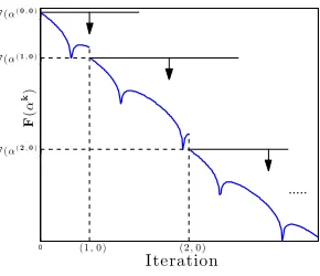
xi∈[0,1]n, (∀i∈[m]) in order to leverage their sparsity. The details of benchmark datasets are shown in Table 1.
5.1 Projection Algorithms
Before presenting the performance of our practical FAPG algorithm, we compared the per-formance of our bisection algorithm (Algorithm 2) against the breakpoint search algorithm (Kiwiel, 2008, Algorithm 3.1) with random pivoting. Both algorithms were implemented in C++. We generated Rn-valued random vectors ˜α with uniformly distributed elements
and computed the projections PSν( ˜α) of ˜α onto Sν, where Sν :=
α | e>
oαo = 12, o ∈ {+,−}, 0 ≤ α ≤ 1
mνe with ν = 0.5. The bisection algorithm used the accuracy of
data m( m+, m−) n range density source
a8a 22,696 ( 5,506, 17,190) 123 [0,1]n 0.113 (Bache and Lichman, 2013)
a9a 32,561 ( 7,841, 24,720) 123 [0,1]n 0.113 (Bache and Lichman, 2013)
australian 690 ( 307, 383) 14 [−1,1]n 0.874 (Bache and Lichman, 2013)
breast-cancer 683 ( 444, 239) 10 [−1,1]n 1.000 (Bache and Lichman, 2013)
cod-rna 59,535 ( 39,690, 19,845) 8 [0,1]n 0.999 (Uzilov et al., 2006)
colon-cancer 62 ( 40, 22) 2,000 [0,1]n 0.984 (Alon et al., 1999)
covtype 581,012 ( 297,711, 283,301) 54 [0,1]n 0.221 (Bache and Lichman, 2013)
diabetes 768 ( 500, 268) 8 [−1,1]n 0.999 (Bache and Lichman, 2013)
duke 44 ( 21, 23) 7,129 [0,1]n 0.977 (West et al., 2001)
epsilon 400,000 ( 199,823, 200,177) 2,000 [−0.15,0.16]n 1.000 (Sonnenburg et al., 2008)
fourclass 862 ( 307, 555) 2 [−1,1]n 0.996 (Ho and Kleinberg, 1996)
german.numer 1,000 ( 300, 700) 24 [−1,1]n 0.958 (Bache and Lichman, 2013)
gisette 6,000 ( 3,000, 3,000) 5,000 [−1,1]n 0.991 (Guyon et al., 2005)
heart 270 ( 120, 150) 13 [−1,1]n 0.962 (Bache and Lichman, 2013)
ijcnn1 35,000 ( 3,415, 31,585) 22 [−0.93,1]n 0.591 (Prokhorov, 2001)
ionosphere 351 ( 225, 126) 34 [−1,1]n 0.884 (Bache and Lichman, 2013)
leu 38 ( 11, 27) 7,129 [0,1]n 0.974 (Golub et al., 1999)
liver-disorders 345 ( 145, 200) 6 [−1,1]n 0.991 (Bache and Lichman, 2013)
madelon 2,000 ( 1,000, 1,000) 500 [0,1]n 0.999 (Guyon et al., 2005)
mushrooms 8,124 ( 3,916, 4,208) 112 [0,1]n 0.188 (Bache and Lichman, 2013)
news20.binary 19,996 ( 9,999, 9,997) 1,355,191 [0,1]n 3.36E-04 (Keerthi and DeCoste, 2005)
rcv1-origin 20,242 ( 10,491, 9,751) 47,236 [0,0.87]n 0.002 (Lewis et al., 2004)
real-sim 72,309 ( 22,238, 50,071) 20,958 [0,1]n 0.002 (McCallum)
skin-nonskin 245,057 ( 50,859, 194,198) 3 [0,1]n 0.983 (Bache and Lichman, 2013)
sonar 208 ( 97, 111) 60 [−1,1]n 1.000 (Bache and Lichman, 2013)
splice 1,000 ( 517, 483) 60 [−1,1]n 1.000 (Bache and Lichman, 2013)
svmguide1 3,089 ( 1,089, 2,000) 4 [0,1]n 0.997 (Hsu et al., 2003)
svmguide3 1,243 ( 947, 296) 22 [0,1]n 0.805 (Hsu et al., 2003)
url 2,396,130 (1,603,985, 792,145) 3,231,961 [0,1]n 3.54E-05 (Ma et al., 2009)
w7a 24,692 ( 740, 23,952) 300 [0,1]n 0.039 (Platt, 1998)
w8a 49,749 ( 1,479, 48,270) 300 [0,1]n 0.039 (Platt, 1998)
Table 1: Details of Datasets. We have scaled the datasets that are highlighted in boldface type.
msec.(#iter.)
Breakpoint Bisection
dim. n range ave. std. ave. std.
100,000 [0,10]n 8.3 (25.7) 2.0 (5.4) 4.9 (31.1) 0.6 (4.7) 100,000 [0,1000]n 9.0 (27.3) 1.4 (4.1) 5.5 (27.1) 1.2 (3.2) 1,000,000 [0,10]n 94.2 (22.6) 16.2 (4.3) 49.9 (32.0) 3.4 (3.1) 1,000,000 [0,1000]n 99.1 (26.5) 15.6 (3.2) 53.4 (30.0) 4.4 (1.5)
101 102 103 104 Number of features n
10−3
10−2
10−1
100
101
102
103
104
105
Time
(sec.)
m=10000,ν=0.5
SeDuMi LIBSVM FAPG LIBLINEAR
103 104 105 Number of samples m
10−1
100
101
102
103
104
105
Time
(sec.)
n=1000,ν=0.5
SeDuMi LIBSVM FAPG LIBLINEAR
0.0 0.2 0.4 0.6 0.8 1.0
ν
10−1
100
101
Time
(sec.)
m=10000, n=100
SeDuMi LIBSVM FAPG LIBLINEAR
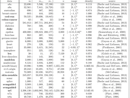
Figure 5: Computation Time forν-SVM
have chosen to use the bisection methods in Section 4.1 to perform the projection steps in Algorithm 4.
5.2 ν-SVM
As mentioned in Section 3.2, the standard C-SVM (11) and ν-SVM (14) are equivalent. Here we chose ν-SVM to solve because choosing the parameter of ν-SVM is easier than that ofC-SVM. We solved theν-SVM (14) via our FAPG method, SeDuMi (Sturm, 1999), and LIBSVM (Chang and Lin, 2011). SeDuMi is a general purpose optimization solver implementing an interior point method for large-scale second-order cone problems such as (14). LIBSVM implements the sequential minimal optimization (SMO) (Platt, 1998) which is specialized for learningν-SVM. For reference, we also compared the FAPG method with LIBLINEAR (Fan et al., 2008) which implements a highly optimized stochastic dual coordinate descent method (Hsieh et al., 2008) forC-SVM3 (Cortes and Vapnik, 1995) and
is known to be quite an efficient method; we note that it may not be a fair comparison because LIBLINEAR omits the bias termbofC-SVM from the calculations,4 i.e., it solves
a less complex model than the ν-SVM (14) in order to speed up the computation.
We terminate the algorithms if the violation of the KKT optimality condition is less than = 10−6. The heuristic option in LIBSVM was set to “off” in order to speed up its convergence for large datasets. In the FAPG method, (ηu, ηd, δ) were set to (1.1,1.1,0.8).
L0 was set to the maximum value in the diagonal elements of Xe>Xe (i.e., the coefficient
matrix of the quadratic form). The initial point α0 was set to the center αc of S ν, i.e.
αc
i = 2m1o,i∈Mo,o∈ {+,−}.
5.2.1 Scalability
First, we compare the computation time with respect to the size of the datasets and pa-rameters using artificial datasets. The results are shown in Figure 5. The left panel shows the computation time with respect to the dimension n of the features form = 10000 and ν = 0.5. The FAPG method has a clear advantage when the dimension n is high, say