Visualizing Minimal Surfaces
Rendering Solid Models with the Aid of 3D
Printers
O. Michael Melko
3D printers are a potentially useful tool for geometric
visualization in mathematical research and education. In this article, we describe the mathematics of minimal surfaces in some detail, and then we present a Mathematica package for generating solid model data of such surfaces. In particular, we show how the package was used to generate a 3D model of Costaʼs surface.
‡
Introduction
In [1], Palais describes a program for the visualization of mathematics through the use of computer graphics. He notes that visualization has been instrumental in some important mathematical discoveries and is also useful for educational purposes. With this in mind, he proposes the creation of an online interactive gallery of mathematical visualization, which he calls a “mathematical exploratorium.” As helpful as computer graphics are for visualization, it can be argued that there is an additional benefit to be had in viewing and handling an actual physical object. Indeed, there has been a long-standing tradition at German universities of producing plaster models of interesting geometric objects. Nowadays, physical models can be easily created by means of stereolithography, or “3D printing technology.”
3D printers produce solid objects from appropriate input data. They were originally cre-ated for rapid prototyping of new product designs but are increasingly being used for other purposes, such as highly customized manufacturing and scientific visualization. Their applications will continue to grow as the underlying technology improves and de-creases in cost. One type of 3D printer uses a powder-binder technology to create objects via a layering technique: a thin layer of powder is spread across a planar surface, and then a print head applies a binder within the cross-sectional area of the object being created. This process is repeated, adding layer upon layer, until the object is complete.
ob-provided. Various file formats may be used to store this data, including the Polygon File Format (or PLY), which is also known as the Stanford Triangle Format. This is the file for-mat used to render Costa’s surface and is described later.
We generate point (or vertex) data for Costa’s surface by means of its Weierstrass represen-tation. Loosely speaking, the Weierstrass representation provides a recipe for creating a parametrization of a minimal surface in 3 from two meromorphic functions defined on a
Riemann surface. In particular, when these functions are ƒ and Cꃣ, where ƒ is the Weierstrass ƒ function and C is a certain constant, the underlying Riemann surface is a torus of the form êG, where G is a discrete lattice in the complex plane . The resulting minimal surface has often been rendered in 3D graphics images. To produce the coordi-nate data for this surface, we must integrate certain rational functions of ƒ and Cꃣ. This results in coordinate functions that are expressed in terms of the Weierstrass ƒ and Ϛ func-tions. Since these functions are built into Mathematica, it is easy to generate the required data.
To generate a solid model, we must produce vertex and face data for a polyhedron that bounds a volume in 3. To achieve this, we first choose a proper subregion of a
fundamen-tal domain of the functions ƒ and Ϛ that contains no poles. This ensures that the corre-sponding piece of Costa’s surface is of finite extent. We then generate two surfaces by means of normal displacement and “glue” the resulting boundaries together. This data is then exported to a PLY file, which is used to print the model.
In what follows, we first provide some background from minimal surface theory. This includes a review of classical surface theory, a description of the Weierstrass represen-tation, a summary of pertinent facts about elliptic functions, and a description of the parametrization of Costa’s surface that we use to generate model data. This is followed by a description of the Minimal Surfaces package developed to render the model data. Then we illustrate how to use the functionality provided by this package to create both graphics objects and PLY data. Finally, discuss some ways in which the work in this paper might be extended, including ideas for mathematical experimentation and enhancements to the Minimal Surfaces package.
‡
A Thumbnail Sketch of Minimal Surface Theory
Intuitively, a smooth surface in Euclidean space 3 is locally area minimizing if any
small deformation of results in a surface of larger area. (The precise mathematical definition of minimal surface requires the introduction of some technical preliminaries and is given later.) Soap films spanning a curve in 3, for example, satisfy this property.
shall discuss Costa’s minimal surface in some detail. We begin by summarizing essential facts from classical surface theory; further details may be found in [2].
·
Essential Facts from Classical Surface Theory
We parametrize a smooth surface in 3 by means of a map X:W Ø, where W is an
open connected subset (or region) in 2, and we assume that XHWL=. We refer to as
the trace of X. Furthermore, we use Hu,vL to denote a system of coordinates on W, and we assume that X is smooth, i.e., differentiable to arbitrary order with respect to u and v. We also assume that X is regular, i.e., that the tangent vectors ∂Xê∂u and ∂Xê∂v are lin-early independent for every point Hu,vLœ W.
Let X,\ denote the standard inner product on 3, and fix an orientation. Then the metric,
or first fundamental form, on with respect to X is given by the symmetric tensor
I:=ds2=E du2+2F du dv+G dv2,
where the coefficients E, F, and G are functions on W given by
E:=[∂X ∂u,
∂X
∂u_,F:=[ ∂X
∂u, ∂X
∂v_,G:=[ ∂X
∂v, ∂X
∂v_.
Let S2 denote the sphere of unit radius in 3 centered at the origin, and let ZHu,vL be the
unit normal vector at the point XHu,vL in that is consistent with the chosen orientation of
3. We use Z`Hu,vL to denote the unique element of S2 that is parallel to ZHu,vL. The map
Z`:W Œ2ØS2Œ3 is called the Gauss map—it provides a measure of how the surface
bends in its ambient space. The Gauss map is used to define the second fundamental form,
II:=L du2+2M du dv+N dv2,
where the coefficients L, M, and N are again functions on W given by
L:= -[∂Z
`
∂u, ∂X
∂u_, M := -[ ∂Z`
∂u, ∂X
∂v_, N:= -[ ∂Z`
∂v, ∂X
∂v_.
We identify the first and second fundamental forms with the 2µ2 symmetric matrices that define them:
I= E F
F G , II=K
L M
M N O.
The forms I and II encode intrinsic and extrinsic geometric properties of the surface . In-trinsic properties are those that are derived from the presence of a distance measure on and do not change under isometric (or distance-preserving) deformations in the ambient space 3. Extrinsic properties are those that depend on how the surface is immersed into 3. (As a motivating example, consider wrapping a geographical map into a tube:
fundamental fact from classical surface theory is that, up to rigid motion, the forms I and II completely determine the geometry of and how it lies in 3.
The mean curvature H and the Gauss curvature K are defined by
(1) H:= 1
2 trIIIÿI -1M= 1
2
L G-2M F+N E
E G-F2 ,
K:=detIIIÿI-1M= L N-M 2
E G-F2.
Both H and K are independent of the choice of coordinates on W, and it turns out that H is an extrinsic property of , while K is an intrinsic property. The latter fact is the well-known Theorem Egregrium of Gauss.
An important example of an intrinsic property of is its area, which we denote by AHL. This area is expressed in terms of the first fundamental form as follows:
(2) AHL:=‡
W
dA=‡
W
detI du dv=‡
W
E G -F2 du dv,
where dA= detI du dv is the infinitesimal element of area on with respect to the parametrization X. Note that the integral in equation (2) is independent of the choice of parametrization, so that it only depends on the trace of X.
Suppose now that r:W Ø is a smooth function. Then we can use r to define a normal variation Xt of M as follows:
XtHu,vL:= XHu,vL+trHu,vLNHu,vL.
For small values of t, the image XtHWL is a smooth surface near = XHWL. If AHtL denotes the area of XtHWL, then a straightforward calculation shows that
A£H0L= -2‡ W
rH dA,
where H and dA denote the mean curvature and element of area of . If a surface is locally area minimizing, we expect the derivative A£H0L to vanish for all choices of r. This can only happen if H vanishes identically. Hence, we have the following:
Theorem. If the surface Œ3 is locally area minimizing, then the mean curvature
H of vanishes identically (Hª0).
The standard definition of minimal surface is motivated by this fact:
Definition: The surface Œ3 is minimal if its mean curvature H vanishes
identically.
The total curvature K of is defined to be
K:=‡
W †K§dA.
We say that has finite total curvature if K< ¶. Furthermore, we say that is complete if all its geodesics can be extended indefinitely. A surface is said to be of finite topological type if it can be smoothly deformed into a compact surface of finite genus, possibly with several holes. It was long conjectured that the only complete, embedded minimal surfaces in 3 of finite topological type are the plane, the catenoid, and the
helicoid. Costa’s minimal surface was the first counterexample to this conjecture to have been found (see [3] for details).
·
The Weierstrass Representation for Minimal Surfaces
It turns out that the geometry of minimal surfaces is intimately related to complex func-tion theory. This connecfunc-tion leads to a simple recipe for constructing minimal surfaces, which we describe here. We only state the necessary results; further details may be found in [2].
We identify 2 with the complex plane by means of the usual correspondence
Hu,vL¨u+i v. Suppose that W is a simply connected region in , that is, a region in in which all closed curves can be contracted to a point. A complex-valued function f on W is said to be holomorphic if its complex derivative f£HzL exists for all zœ W.
Theorem. Suppose that f,g:W Ø are two holomorphic functions on a simply
con-nected region W, and define y:W Ø3 to be the holomorphic curve with components
(3)
y1HzL:= fHzL
4 I1-gHzL
2M,
y2HzL:=i fHzL
4 I1+gHzL
2M,
y3HzL:= 1
2 fHzLgHzL. Then we have the following: (i) Componentwise integration
(4)
gHzL:=‡
z0 z
yHzLdz
yields a holomorphic curve g:W Ø3.
(ii) For each tœ, the trace of the map
is a minimal surface. The collection of all such maps is called the associate family of g. (iii) For any tœ, g is the stereographic projection into of the Gauss map of Xt.
Since f and g are assumed to be holomorphic on W, and W is assumed to be simply con-nected, it follows from basic complex function theory that the integration in equation (4) is path independent.
We refer to a triple Hf,g,WL satisfying the above conditions as the Weierstrass data for the corresponding associate family XtHWL, and we refer to X0 as the Weierstrass
representa-tion of the minimal surface :=X0HWL. Note that Xt is an isothermal parametrization for each tœ, that is, the coefficients of the first fundamental form satisfy E=G and F=0. In fact, it can be shown that
(6) ds2= 1
4»»fHzL »»
2I1+»»gHzL »»2M2»»dz»»2,
where z=u+i v. Also, we have
(7)
K= -16»»g
£HzL »»2
»»fHzL »»2I1+»»gHzL »»2M4 .
Here, »»z»» denotes the complex norm of z and »»dz»»2 =du2+dv2.
·
Meromorphic Functions on Complex Tori
Our goal in this subsection is to introduce the Weierstrass data used to obtain a parametrization of Costa’s surface. Before doing so, we provide a little background in ellip-tic function theory. Details may be found in [4].
Suppose that w1 and w2 are two complex numbers such that Im@w1êw2D≠0. Then the lat-tice of points G:=8k1w1+k2w2 k1,k2œ< is a subgroup of the group of translations
on and G is isomorphic to the additive group of Gaussian integers @iD. Thus, w œ G
acts on by the rule zØz+ w, and the quotient space êG is topologically a torus, which inherits a complex structure from . Let p:ØêG denote the corresponding pro-jection map. We refer to w1 and w2 as basic periods of G and sometimes write T for êG.
Any function f` on êG lifts to a function f on . Such a function satisfies fHz+ wL= fHzL for all w œ G and is said to be G periodic. It is not possible for a complex function to be both G periodic and holomorphic in all of , but there is a rich theory of functions that are
G periodic and meromorphic. A function f is meromorphic on W if it is holomorphic on
W\A, where A is a discrete set without accumulation points in W, and if, for any aœA, f has a pole at a, that is, f has a power series expansion in a neighborhood of a of the form
fHzL= c-k
Hz-aLk ++ c-1
z-a +c0+c1Hz-aL+c2Hz-aL
The positive integer k is called the order of the pole at a. A pole is said to be simple if it is of order one. Functions that are both meromorphic and periodic with respect to some lat-tice G are referred to as elliptic functions.
Our objective in what follows is to describe a particular solution of the period problem. In the context of complex tori, it may stated as follows:
The Period Problem: Find meromorphic functions f and g, periodic with respect to
some lattice G in , such that Re@gD is also G periodic, where g is given by equation (4). Here, the Weierstrass data is Hf,g,W\AL, where W is a fundamental domain of G in , and A is the set of poles of f and g in W.
Note that, by making appropriate cuts in W\A, we may consider it to be simply connected. Any solution to this problem will topologically be a torus (possibly with several holes) im-mersed in 3.
Costa’s surface arises from what is arguably the most basic of elliptic functions: the Weier-strass ƒ function. It is defined by the series expansion
(8)
ƒHz;GL:= 1
z2 + ‚
w œ G*
: 1
Hz- wL2
-1
w2>,
where G* := G\80< denotes the set of nonzero elements in G. This function has poles of or-der two at each of the lattice points in G and is holomorphic everywhere else in . It there-fore projects to a meromorphic function with exactly one pole of order two in êG. It is known that any meromorphic function on êG may be expressed as a rational function of
ƒHz;GL and its complex derivative ƒ£Hz;GL. In fact, these functions are related by the funda-mental equation
(9)
ƒ£Hz;GL2=4HƒHz;GL-e
1L HƒHz;GL-e2L HƒHz;GL-e3L,
where
(10) e1:= ƒK
w1
2 O, e2:= ƒK
w2
2 O, e3:= ƒ
w1+ w2
2 .
A related function is the Weierstrass Ϛ function, which is defined by
(11) ϚHz;GL:= 1
z +w œ G*‚ : 1
z- w+
1
w +
z
w2>.
The Ϛ function is not G periodic and hence not elliptic. It is holomorphic on \G, how-ever, and has simple poles at the points of G. Furthermore, it is related to the Weierstrass
ƒ function by the rule
(12) Ϛ£Hz;GL= -ƒHz;GL.
(13) ϚHz+ wk;GL=ϚHz;GL+2ϚKwk
2 ;GO, k=1, 2. Furthermore, a theorem due to Legendre states that
(14)
w2ϚKw1
2 ;GO- w1ϚK
w2
2 ;GO= pi. These facts are used in the next subsection.
We refer to special points in or êG as marked points. These are points at which singu-larities, such as poles, occur. Open disks centered at marked points are referred to as marked disks. Let DHz,εL denote the disk of radius ε with center at the point zœ, and de-fine DGHz,εL by
DGHz,εL:=DHz,εL+ G =8x+ w xœDHz,εL,w œ G<.
The set DGHz,εL can be viewed as the collection of all points in that are mapped to a marked disk in êG by the projection p.
We now specialize to the case where w1=1 and w2=i. In this case, G is the standard square lattice of Gaussian integers in , and we simply write ƒHzL for ƒHz;GL and ϚHzL for ϚHz;GL. The numbers in equation (10) now satisfy
(15) e1= -e2, e3=0.
The set U:=8u+i v 0bu,vb1< defines a fundamental domain of the covering
p:ØêG. Let
B=DGH0,ε1L ‹DGH1ê2,ε2L ‹DGHiê2,ε3L,
where ε1, ε2, and ε3 are small positive numbers, and define WHε1,ε2,ε3L to be U\B. Note that WHε1,ε2,ε3L is a unit square in with four quarter-disks of radius ε1 removed from the corners of U, two half-disks of radius ε2 removed from the midpoints of the horizontal edges of U, and two half-disks of radius ε3 removed from the midpoints of the vertical
edges of U. The projection pHU\BL is a torus with three marked disks removed. These disks are centered at pH0L, pH1ê2L, and pHiê2L.
With these preliminaries, we are ready to specify the Weierstrass data for Costa’s surface. We take our domain to be WHε1,ε2,ε3L, and set
(16) fHzL= ƒHzL, gHzL= 8pe1
ģHzL .
Both of these functions are holomorphic on WHε1,ε2,ε3L, and since WHε1,ε2,ε3L is simply
connected, the integration in equation (4) is path independent.
·
Costa
ʼ
s Minimal Surface
In general, one might have to resort to numerical integration in equation (4) to obtain the Weierstrass representation for a surface. However, the integration can be carried out explic-itly for the functions in equation (16), when restricted to WHε1,ε2,ε3L. This calculation
itly for the functions in equation (16), when restricted to WHε1,ε2,ε3L. This calculation was first performed by Alfred Gray and is given in [2]. The result is as follows:
Theorem. Let G@1ê2D:=8k1w1+k2w2 2k1, 2k2œ< denote the lattice of Gaussian half-integers. Then the Weierstrass data in equation (16), when substituted into equation (3) and integrated, yields the holomorphic curve g:\G@1ê2DØ3, whose components are given by
(17)
g1HzL:= 1
2:-ϚHzL+ pHz-iL+
p2H1+iL
4e1 >+
p
4e1 :Ϛ z -1
2 -Ϛ z -i
2 >,
g2HzL:= i
2:-ϚHzL- pHz-1L
-p2H1+iL
4e1 > -ip
4e1 :Ϛ z -1
2 -Ϛ z -i
2 >,
g3HzL:= 2p
4 :log
ƒHzL-e1
ƒHzL+e1 -ip>.
The corresponding trace of X0=Re@gD is Costa’s minimal surface.
We now use the properties of ƒ and Ϛ discussed earlier to demonstrate that Costa’s surface is topologically a torus with three points removed. Define three points in
:=êG by a1:= pH0L, a2:= pH1ê2L, and a3:= pHiê2L . We may think of these points as the projection to of G@1ê2D in . From the form of g in equation (17), it is clear that
g is holomorphic on \G@1ê2D.
Note that, for the basic periods H1,iL, we have iG = G as sets. In this case, it is clear from the definition of the Ϛ function in equation (11) that
ϚHi z;GL=ϚHi z;iGL= 1
i ϚHz;GL.
This fact, together with equation (14), implies that
(18) Ϛ 1
2 =
p
2, Ϛ i
2 =
-pi
2 .
Equations (13, 17, 18) then allow us to conclude that
gHz+1L= gHzL+ipH1, 0, 0L, gHz+iL= gHz+iL+ipH0,-1, 0L.
This clearly implies that Re@gHz+ wLD=Re@gHzLD for all w œ G, that is, that X0 is G peri-odic. Thus, we have demonstrated the following:
Proposition: The map X0=Re@gD, where g is given by equation (17), solves the period problem. Hence X0 projects to a real-analytic map X
`
0:\8a1,a2,a3<Ø3.
(19) ds2= 1
4 »»ƒHzL »»+
2p»»e1»»
»»ƒHzL2-e 12»»
2
»»dz»»2.
From this formula, it is not difficult to show that the function dsê »»dz»» has poles of order two at a1, a2, and a3. Thus, the metric diverges at the ends of Costa’s surface, which we define to be the image under X`0 of the punctured disks pHD£H0,εLL, pHD£H1ê2,εLL, and
pHD£Hiê2,εLL in . Here, D£Hz,εL denotes the disk DHz,εL in , excluding its center. We shall see later that X`0 diverges at different rates at a1 than at a2 and a3. This is due to the fact that the principal part of the Laurent expansion of dsê »»dz»» at z=0 has a larger lead-ing coefficient than that at z=1ê2 or z=iê2, even though all of the poles are of the same order. As can be seen in Figure 3, the end corresponding to the punctured disk about
a1= pH0L is asymptotically planar, while the other two ends are asymptotically catenoidal in form.
In the next section, we describe the contents of the Minimal Surfaces package. After that, we show how to use the package to generate polyhedral data representing the trace of the parametrization
(20) X`0:W`Hε1,ε2,ε3LØ3,
where W`Hε1,ε2,ε3L:= p@WHε1,ε2,ε3LD.
‡
The Minimal Surfaces Package
We now describe the public functions in the Minimal Surfaces package. Note that there are a number of utility functions with private context that are not described here. Further documentation may be found within the package source file.
·
Special Data Types
Arc@8x, y<, r, 8q1, q2<, orientationD is a two-dimensional graphics primi-tive specifying a circular arc with center 8x,y<, radius r, and initial and terminal angles 8q1,q2<, which are assumed to satisfy -p § q1,q2§ p. The orientation may be either
Clockwise or CounterClockwise.
·
Surface-Generating Functions
CostaSurface@u, vD returns the image in 3 corresponding to the point in 2ï2
ParallelSurface@X, p, dD returns the normal displacement at distance d from XHpL along the normal of X at XHpL, where X is a regular map on some domain W Œ2
into 3.
·
Vertex Creation and Triangulation
CreateVertexData@curve, optionsD produces a collection of planar points
within the boundary specified by the closed curve curve=8c1,c2, …<, which consists of a list of line segments and circular arcs and is assumed to be traversed counterclockwise.
The output is a list of the form 8interior,boundary<. The interior list consists of planar points properly inside the boundary specified by curve, while boundary =8b1,b2,…< is a list of sublists, each member of which is a list of planar points lying on the corresponding line segment or arc specified by curve.
Currently, the only supported option is MeshSizeØ8n1, n2<, which specifies the
num-ber of sample points to use in the x and y directions. The defaults are n1=n2=10.
GlueComponents@top, bottomD glues together a pair of polyhedral surfaces
speci-fied by the lists top and bottom. These lists are assumed to have the same form 8vertices, faces,boundary< as output from the Triangulate function. It is also as-sumed that the boundary components of top and bottom have the same shape.
The output has the form 8vertices, faces<, where vertices is the join of the vertex sublists of top and bottom, and faces is a list of sublists of the form 8top- faces,bottom- faces,boundary- faces<.
Triangulate@vertices, curve, optionsD produces a triangulation of a planar
region. The list vertices is of the same form as the output of CreateVertexData, and curve, which consists of a list of line segments and circular arcs, defines the boundary of the region to be triangulated.
The output is a list of the form 8vertices, faces,boundary<. The elements of vertices are planar points of the form 8x,y<. The elements of faces are ordered triples of positive inte-gers 8a,b,c<. The elements of such triples refer to positions in the list of vertices and thereby define triangles. The list boundary is of the form 8p1, p2, …<, where each sublist
pj contains positive integers pointing to the position in the list vertices of points that lie on the jth connected component of the boundary of the triangulated region.
This function has one option, which is of the form IdentificationsØl. The default value for l is l=8<, in which case no identifications occur. The other possibility is l=8l1,l2<, where each element of l1 specifies the positions of a pair of edges in curve that are to be
Remark: The result after identification is assumed to be a Riemann surface, possibly with several marked disks removed.
·
Graphics Functions
CreatePolyhedron@8vertices, faces<D returns a list of 3D graphics
direc-tives and primidirec-tives describing a polyhedron. The sublist vertices consists of points that are the vertices of a polyhedron, and faces is a list of sublists of the form 8x1,x2, …<, where xj has the form 9gj, fj=. Each gj is a list of graphics directives to be applied to the face list fj.
Remark: This function could easily be modified to allow the application of graphics directives to edges and vertices.
·
Import/Export Functions
ExportGraphics@"file", data, "format"D writes geometric data contained
in the list data to an ASCII file named file. The list data is assumed to be in the same form as input data to CreatePolyhedron, except that Mathematica graphics direc-tives are replaced with equivalent direcdirec-tives that are compliant with the export format. The form of the output is specified by format. Currently the only supported format is PLY, which stands for the polygon file format
Remark: A desirable enhancement to this function would be to include a POVRAY export format. This would produce object data appropriate for creating scenes with the Per-sistence of Vision Raytracer program.
·
The Polygon File Format
We now give a brief summary of the PLY file format, limiting our discussion to those as-pects used in the current version of the ExportGraphics function. Further details may be found in [5].
element vertex 8 property float32 x property float32 y property float32 z
specifies that the file in question contains data for eight vertices and that each vertex has three properties Hx,y,zL, which are floating-point numbers representing the coordinates of the vertex.
Each line of the vertex list specifies the Hx,y,zL coordinates of a vertex. A list of data speci-fying faces follows the vertex data. Each line of this list gives, in order, the number of ver-tices in a face and the position in the vertex list corresponding to a vertex of the face. Color attributes of the face can then be given in the form of RGB-color intensities, which are specified by integers from 0 to 255. The orientation of a face can be determined from the order in which its vertices are presented. Note that indexing of the vertices begins at 0. Thus, when 0 occurs in the vertex list of a face in Listing 1, for example, it points to the first vertex, which has coordinates H0, 0, 0L.
ply
format ASCII 1.0
comment a cube a comment
element vertex 8 8 vertices in file
property float32 x x coordinate of vertex
property float32 y y coordinate of vertex
property float32 z z coordinate of vertex
element face 6 6 faces in file
property list uchar int vertex_indices vertex incidence list
property uchar red property uchar green property uchar blue end header
0 0 0 start of vertex list
0 0 1 0 1 1 0 1 0 1 0 0 1 0 1 1 1 1 1 1 0
4 0 1 2 3 128 0 128 start of face list
4 7 6 5 4 192 128 0 4 0 4 5 1 128 192 0 4 1 5 6 2 256 0 0 4 2 6 7 3 0 256 0 4 3 7 4 0 0 0 256
·
A Note on Performance
Of the functions listed above, the most time-consuming is Triangulate, which inter-nally calls DelaunayTriangulation. It seemed convenient to use the latter because it is part of the ComputationalGeometry package, which is a standard Mathematica add-on package. Another attractive feature of Delaunay triangulation is that, by design, it produces the most regular triangulation of a planar point set. The most efficient algo-rithms for Delaunay triangulation have a time complexity of OHnlogHnLL.
The model shown in Figure 4 was created by evaluating Triangulate on a vertex set containing about 60,000 points. This took more than 14 hours on a workstation with dual Opteron 244 processors. (Mathematica Version 5.2 only used one CPU, and the availabil-ity of RAM was not an issue.)
There are at least two ways the overall performance of the Minimal Surfaces package could be improved, both of which involve reducing the vertex data used as input to
Triangulate. This is discussed further in the subsection on enhancements.
We note that an alternative approach might be to replace the current version of
Triangulate with an “adaptive cell division algorithm.” In this scenario, one would
start with a sparse vertex set in the given domain W, which would be triangulated by some method. Then one would use some function, such as the metric in equation (6), to decide if the triangulation needs to be refined in a neighborhood of any given vertex. The best method of refinement is likely to be midpoint subdivision of any triangle incident to the vertex in question. This may prove to be faster than using Delaunay triangulation.
‡
Generating the Model Data for Costa
ʼ
s Surface
We now show how the functions described above are used to create a model of Costa’s sur-face. The essential steps are as follows:
1. Use the Line and Arc data types to define a curve bounding a suitable domain
W Œ.
2. Call CreateVertexData to obtain a collection of points VΠW.
3. Apply Triangulate to V in order to obtain its Delaunay triangulation; provide boundary identifications, if appropriate.
4. Apply a composition of ParallelSurface and CostaSurface to the data V generated in step 2 to obtain vertex data for two polyhedral surfaces in 3 that
are normal displacements of points lying on Costa’s surface. Note that the faces of the resulting polyhedral surfaces are defined by the same incidence relations result-ing from step 3.
5. Use GlueComponents to create a single volume-bounding polyhedron from the
two normally displaced polyhedral surfaces created in step 4.
6. Call ExportGraphics to produce the PLY file required for printing a solid model.
First, we load the Minimal Surfaces package and define some useful functions. It is avail-able from www.mathematica-journal.com/data/uploads/2010/12/MinimalSurfaces.m. We assume the package is contained in the same directory as this article.
SetDirectory@NotebookDirectory@DD; <<MinimalSurfaces`
The following function defines the curve bounding the region WHd,e,fL described in the paragraph after equation (15). Recall that the input parameters Hd,e,fL represent the radii of the three marked disks with centers at pH0L, pH1ê2L, and pHiê2L, where p, as before, de-notes the projection p:ØêG. Note that this curve consists of 16 segments and is tra-versed counterclockwise, hence the circular arcs it contains are tratra-versed clockwise.
boundary@d_, e_, f_D:=8
Line@88d, 0<, 8H1ê2L- e, 0<<D,
Arc@81ê2, 0<, e, 8p, 0<, ClockwiseD, Line@88H1ê2L+ e, 0<, 81- d, 0<<D, Arc@81, 0<,d, 8p, pê2<, ClockwiseD,
Line@881,d<, 81, H1ê2L- f<<D,
Arc@81, 1ê2<, f, 8- pê2,pê2<, ClockwiseD, Line@881,H1ê2L+ f<, 81, 1- d<<D,
Arc@81, 1<,d, 8- pê2, - p<, ClockwiseD,
Line@881- d, 1<, 8H1ê2L+ e, 1<<D, Arc@81ê2, 1<, e, 80, - p<, ClockwiseD, Line@88H1ê2L- e, 1<, 8d, 1<<D,
Arc@80, 1<,d, 80, - pê2<, ClockwiseD,
Line@880, 1- d<, 80, H1ê2L+ f<<D,
Arc@80, 1ê2<, f, 8pê2, - pê2<, ClockwiseD, Line@880,H1ê2L- f<, 80,d<<D,
Arc@80, 0<,d, 8pê2, 0<, ClockwiseD <
The function grid generates a rectangular array of horizontal and vertical lines with off-set q=8q1,q2<, step size s=8s1,s2<, and index range n =88n11,n12<,8n21,n22<<; it is used
gridlines@q_, s_, n_D:= Join@
Table@
Line@88qP1T +k sP1T, qP2T+nP2TP1TsP2T<, 8qP1T+k sP1T, qP2T+nP2TP2TsP2T<<D, 8k, nP1TP1T, nP1TP2T<
D,
Table@Line@88qP1T+nP1T P1TsP1T, qP2T+k sP2T<, 8qP1T+nP1T P2TsP1T, qP2T+k sP2T<<D,
8k, nP2TP1T, nP2TP2T<D D;
·
Example Output from CreateVertexData and Triangulate
Before invoking the commands that produce the graphics object illustrated in Figure 3, we illustrate what the output of the CreateVertexData and Triangulate functions looks like for a small mesh size.
b=boundary@1ê6, 1ê4, 1ê4D;
v=CreateVertexData@b, MeshSizeØ810, 10<D;
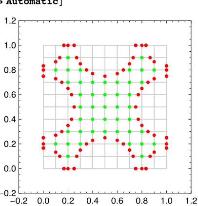
The list v produced is of length 2. The first part of v consists of the interior points shown in green in Figure 1. Here is a short listing.
vP1T êêShort
:: 1
10, 1
5>, á43à, : 9
10, 4
5>>
The second part of v consists of 16 sublists, each of which contains vertices that lie on the corresponding segment of b. For example, the last segment in b corresponds to the quar-ter-circle in the lower-left corner of Figure 1. The vertices that lie in the segment bP-1T are the elements of the list vP2, -1T.
vP2, -1T
::0, 1 6>, :
1
10, 2
15>, : 2
15, 1
10>, : 1
6, 0>>
vP2, 1T
::1
6, 0>, : 1
5, 0>,: 1
4, 0>>
Figure 1, below, graphically illustrates the structure of v. The green points are vertices that lie in the interior of the boundary curve b, and the red points are vertices lying in b it-self. Note that all of the points in v lie in the gray rectangular grid.
Show@ Graphics@
[email protected]`D, gridlines@80, 0<, 80.1`, 0.1`<, 880, 10<, 80, 10<<D<,
8Green, [email protected]`D, PointêüvP1T<,
8Red, [email protected]`D, PointêüFlatten@vP2T, 1D<<D, FrameØTrue, PlotRangeØ88-0.2`, 1.2`<, 8-0.2`, 1.2`<<, AspectRatioØAutomaticD
-0.2 0.0 0.2 0.4 0.6 0.8 1.0 1.2
-0.2 0.0 0.2 0.4 0.6 0.8 1.0 1.2
Ú Figure 1. Vertex data generated using CreateVertexData with parameter values d =1ê6,
e = f =1ê4, and MeshSizeØ810, 10<.
We now triangulate the vertex data v shown in Figure 1 without edge identifications. The resulting triangulation differs from a Delaunay triangulation in that certain triangles inci-dent to boundary points of WHd,e,fL but not lying within the domain itself are excluded.
p=Triangulate@v, bD;
pP1T êêShort
:: 1
10, 1
5>, á111à, : 2
15, 1
10>>
The second part of p contains incidence relations that define faces, which are always trian-gles. The positive integers in each sublist of pP2T are locations of vertices in pP1T.
pP2T êêShort
881, 109, 110<, á154à, 845, 77, 78<<
For example, the following command extracts the vertices in pP1T that correspond to the first face listed in pP2T.
Part@pP1T, pP2, 1TD
:: 1
10, 1
5>, :0, 1
4>, :0, 1
5>>
The third part of p is a list containing one sublist pP3, 1T that defines the boundary curve of the triangulation. When identifications are used, the list pP3T may contain multi-ple boundary components. In the next subsection, for exammulti-ple, Triangulate is called with identifications that produce three boundary components. Each component in that case corresponds to the boundary of a marked disk that has been removed from the torus
described in the paragraph after equation (17).
pP3T êêShort
8846, 47, 48, 49, á60à, 110, 111, 112, 113<<
The following group of commands first maps the vertices of p into the horizontal plane of
3; the resulting output list is named q. Then some graphics directives are added to q, and
the resulting list is used as input to CreatePolyhedron. The output list s is then flat-tened so that it can be used as input to Graphics3D.
id@u_, v_D:=8u, v, 0<
q=8Apply@id, pP1T, 81<D, pP2T, pP3T<;
gr=:RGBColorB3 4,
3
4, 0F, Specularity@GrayLevel@1D, 5D>; qw=8qP1T, 88gr, qP2T<<<;
s=CreatePolyhedron@qwD; ss=Flattenêüs;
of sP1T consists of graphics directives, and the second part consists of graphics primi-tives that are applied to the faces of the triangulation q. Part of the output from the current evaluation is shown below. To create the polyhedron shown in Figure 3, we will build a list similar to qw, above. The second part of the resulting list itself has five parts, each of which corresponds to one of the five parts of the surface shown in the figure, namely, the green (or inside) part, the yellow (or outside) part, and the three purple rims.
sP1, 1T
:RGBColorB3
4, 3
4, 0F, Specularity@GrayLevel@1D, 5D>
sP1, 2, 1T
PolygonB:: 1
10, 1
5, 0>, :0, 1
4, 0>, :0, 1
5, 0>>F
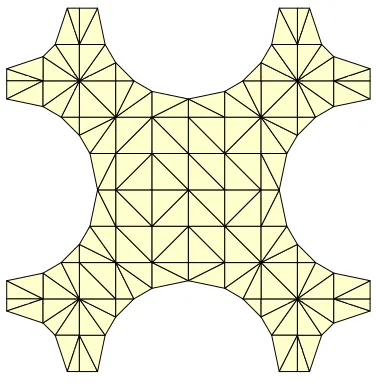
Figure 2 shows what the triangulation of the small dataset looks like.
Show@Graphics3D@ssD, AspectRatioØAutomatic, AxesØFalse, BoxedØFalse, ViewPointØ80, 0, 9<D
Ú Figure 2. Triangulation of the vertex data in Figure 1 using the Triangulate function.
·
Creation and Triangulation of Vertex Data for a Torus
resulting datasets. Note that our marked disks are given radii of d =1ê8 and
e = f =1ê24. This compensates for the difference in the rate of divergence at the poles
pH0L, pH1ê2L, and pHiê2L of the parametrization X`0 defined in the proposition following
equation (17). The ends of the resulting surface are roughly the same size.
b=boundary@1ê8, 1ê24, 1ê24D;
v=CreateVertexData@b, MeshSizeØ850, 50<D;
The list edgeIds specifies edges in b that are to be identified, and the list vertexIds
specifies the endpoints of circular arcs in b that are to be identified. For example, the sub-list 81, 11< in edgeIds indicates that the lower-left horizontal line segment in Figure 2 is to be identified with the upper-left horizontal line segment. Similarly, the sublist 82, 10< in
vertexIds indicates that corresponding endpoints of the semicircular arcs with centers
at H1ê2, 0L and H1ê2,iL are to be identified. The list vertexIds is used to identify which components of the boundary curve close up to form boundary curves. In this case, we get three such curves.
edgeIds = 881, 11<, 83, 9<, 85, 15<, 87, 13<<; vertexIds = 882, 10<, 84, 16, 12, 8<, 86, 14<<;
When we pass these identifications to Triangulate as an option, output similar to that in the previous subsection is produced, except that some incidence relations in p are reas-signed, and extra vertices are dropped.
p=Triangulate@v, b, Identifications Ø8edgeIds, vertexIds<D;
·
Vertex Data for Normal Displacements of Costa
ʼ
s Surface
The ParallelSurface function is used to create a small normal offset of the
vector-valued function it takes as an argument. Here, the function is CostaSurface, which can be used to generate the true Costa surface. Note that, since CostaSurface returns a vector in 3, ParallelSurface also returns a vector in 3.
Z@u_, v_, rho_D:=
ParallelSurface@CostaSurface@x, yD, 8x, y<, rhoD ê. 8xØu, yØv, dØrho<
To create the polyhedron in Figure 3, we choose r =±0.025 as our offset and define two real vector-valued functions accordingly.
X1@u_, v_D:=Re@Z@u, v, 0.025DD X2@u_, v_D:=Re@Z@u, v, -0.025DD
q1=8Apply@X1, pP1T, 81<D, pP2T, pP3T<; q2=8Apply@X2, pP1T, 81<D, pP2T, pP3T<;
The function GlueComponents is now used to connect the boundary components of
q1 and q2. First, the vertex and face lists of q1 and q2 are concatenated, and then addi-tional faces, which are incident to vertices in the boundary curves, are appended to the face list. The resulting polyhedron bounds a volume in 3.
zx =GlueComponents@q1, q2D;
We now define the graphics directives we wish to apply to each component of our surface.
gr1=:EdgeForm@D, RGBColorB1 2,
3
4, 0F, Specularity@[email protected]`D, 6D>;
gr2=:EdgeForm@D, RGBColorB3 4,
1
2, 0F, Specularity@GrayLevel@1D, 9D>;
gr3=:EdgeForm@D, RGBColorB1 2, 0,
1
2F, Specularity@GrayLevel@1D, 9D>;
The following command produces input in the form required by CreatePolyhedron. That is, qw has the form qw=8verts, 88g1, f1<, …, 8gn, fn<<<, where each fj is a list of incidence relations in the vertex list verts defining faces and each gj is a list of graphics directives to be applied to fj.
qw = 8zxP1T, Join@88gr1, zxP2TP1T<,8gr2, zxP2TP2T<<, Map@8gr3, Ò<&, zxP2TP3TDD<;
Now we apply CreatePolyhedron to get a graphics object. As before, we need to flat-ten the list s to produce input acceptable to the Graphics3D function.
Graphics3D@ss, AspectRatioØAutomatic, AxesØFalse, BoxedØFalse, LightingØ"Neutral",
ViewPointØ8-2.417`, -1.984`, 1.294`<D
Ú Figure 3. Costaʼs surface with d =1ê8, e = f =1ê24, r =±0.1, and MeshSizeØ850, 50<.
·
Printing Technology and the Solid Model
The photograph shown in Figure 4 is a 3D model of Costa’s surface that was printed using a ZCorp Model 402Z 3D printer. This device is no longer in production but is similar to the ZCorp Model 510. The principal difference between the two is that the Model 510 has a higher print resolution. See [6] for more details on the Model 510.
We first convert our choice of RGB values to integers in the range @0, 255D.
rgb=
Floor@256881ê2, 3ê4, 0<, 83ê4, 1ê2, 0<, 81ê2, 0, 1ê2<<D;
Now we produce a list rw in the correct format for input into the ExportGraphics
function. Note its similarity in structure to qw.
rw = 8zxP1T, Join@88rgbP1T, zxP2TP1T<, 8rgbP2T, zxP2TP2T<<, Map@8rgbP3T, Ò<&, zxP2TP3TDD<;
The PLY file corresponding to the surface pictured in Figure 3 is produced by invoking
the ExportGraphics function as follows.
ExportGraphics@"costa-8-24-24-50-50.ply", rw, "PLY"D
To obtain the solid model illustrated in Figure 4, a PLY file was created using the parame-ters d =1ê8, e = f =1ê24, r =±0.2, and MeshSizeØ8250, 250<. The large mesh size ensured that the model would be smooth, and the rather large normal displacement
size ensured that the model would be smooth, and the rather large normal displacement
r =±0.2 ensured that it would be thick enough to avoid breakage during production. The resulting object is about eight inches in diameter.
Ú Figure 4. Photograph of a solid model of Costaʼs surface generated from a PLY file with parame-ters d =1ê8, e = f =1ê24, r =±0.2, and MeshSizeØ8250, 250<.
‡
Discussion
In this section, we put what was done here in perspective and outline some ways of generat-ing Weierstrass data that may lead to new examples of minimal surfaces. These methods, together with other enhancements discussed in this section, may be incorporated in future versions of the Minimal Surfaces package.
·
Genus One Minimal Surfaces
First, it would be interesting to look for other examples of genus one minimal surfaces, pos-sibly with more than three ends. The Weierstrass data for such a surface would be given by elliptic functions on . An obvious choice for Weierstrass data would be
(21) fHzL= ƒkHz;GL, gHzL= C
ƒk£Hz;GL,
where C is a constant, and ƒkHz;GL, for k¥2, is defined on êG by the absolutely conver-gent series
ƒkHz;GL:= 1
zk + ‚
w œ G* 1
Hz- wLk -1
The case k=2 is just that of Costa’s surface, where G =@iD and C= 8pe1. The
con-vergence of this series is actually rather subtle for k=2, and the difference in the sum-mands cannot be separated. For k¥3, we may rewrite ƒkHz;GL as
ƒkHz;GL= H-1L
k-2
k!
dk-2
dzk-2 ƒHz;GL+EkHGL,
where EkHGL is the Eisenstein series of weight k:
EkHGL:= ‚ w œ G*
1
wk.
It was mentioned earlier that any elliptic function may be expressed as a rational function of ƒHz;GL and its derivative ƒ£Hz;GL. We can achieve this for the Weierstrass data in equa-tion (21) by repeatedly differentiating equaequa-tion (9) and applying the above observaequa-tions.
·
Higher Genus Minimal Surfaces
We now discuss two ways in which one may generate examples of minimal surfaces that have a topology other than that of a torus.
ü Automorphic Functions on Hyperbolic Space
Every compact, connected surface has a simply-connected universal covering space, which we denote by *. If has no additional structure, we know that * must be topologi-cally a sphere, which we take to be the extended complex plane ‹ 8¶<, or an open sub-set of the plane, which we take to be . A surface is said to have a conformal structure if, for every point pœ, one has a notion of the angle between any two tangent vectors based at p. If is a simply connected region in , we have the following fundamental fact from complex analysis:
Riemann Mapping Theorem. Any simply connected region in the complex plane
(other than itself) is conformally equivalent to the unit disk U:=8zœ z <1<. A Riemann surface is a surface endowed with a conformal structure. If is a Riemann surface of genus at least two, the Riemann mapping theorem allows us to think of its uni-versal covering space * as being the unit disk UŒ. In fact, following [7], a simply con-nected Riemann surface * is classified as being
Ë elliptic if it is conformally equivalent to the whole Riemann sphere ‹ 8¶<
Ë parabolic if it is conformally equivalent to the finite plane Ë hyperbolic if it is conformally equivalent to the unit disk U
Ë If * is elliptic, then is the full group of linear fractional transformations zØHa z + bL ê Hc z +dL for complex constants a, b, c, and d with a d-b c≠0.
Ë If * is parabolic, then is the group of linear transformations zØa z+ b, for complex constants a and b.
Ë If * is hyperbolic, then is the group of linear fractional transformations of the form zØeiqHz -aL ë H1-āzL, where q œ, aœU, and ā is the complex conju-gate of a. In this case, is isomorphic to the matrix group PSL2HL.
In accordance with the above, we say that is elliptic if * is elliptic, is parabolic if * is parabolic, etc. To simplify the discussion a bit, we sometimes use the term Weierstrass data to mean a pair of meromorphic functions Jf`,g`N on a compact Riemann surface .
These functions lift naturally to a pair of G-invariant functions Hf,gL on *.
The catenoid is an example of a minimal surface that arises from Weierstrass data on an el-liptic Riemann surface. The main subject of this paper has been Costa’s surface, which arises from Weierstrass data on a parabolic Riemann surface (i.e., a torus). Minimal sur-faces of higher topological type arise from Weierstrass data on Riemann sursur-faces of hyper-bolic type. In order to find such data, we seek meromorphic functions Hf,gL on the unit disk U that are invariant under a discrete subgroup G Œ. Such functions are referred to as automorphic functions. A fundamental domain of G acting on U can be specified by a subregion of U bounded by line segments and circular arcs. Thus, the rendering methodol-ogy used here should extend directly to the hyperbolic case. This leads us to pose the following:
Problem: Use automorphic functions on the unit disk U as Weierstrass data for the con-struction of new examples of minimal surfaces.
It should be noted that the author has not been able to find any references in the mathemati-cal literature taking this approach to the construction of minimal surfaces. There is an-other approach, however, which is briefly discussed in the next section.
ü Algebraic Curves in 2
Riemann surfaces may also be realized as affine algebraic curves in 2, which are the solu-tions of polynomial equasolu-tions in two complex variables of the form PHz,wL=0. Such curves are not compact, but they can be compactified via an embedding into the complex projective plane P2. From this perspective, Riemann surfaces can easily be identified with branched coverings of the complex plane or the Riemann sphere ‹ 8¶<. In equa-tion (9), for example, we see that the Weierstrass data for Costa’s surface essentially pro-vides a complex parametrization of the elliptic curve
w2=4z3-g2z-g3,
where g2:= -4He1e2+e1e3+e2e3L and g3:=4e1e2e3.
Gackstatter–Karcher surfaces or CGK surfaces. In constructing these surfaces, he first identifies Riemann surfaces of the form
wk-RHzL=0,
where RHzL is a rational function in z of a specific form. He then constructs minimal sur-faces with the Weierstrass data fHzL=1 and gHzL=C wk-1=C RHzLHk-1Lêk, which are
de-fined on a specific branch of the underlying Riemann surface. Here, the Gauss map g may be viewed as a multivalued function from into the Riemann sphere ‹ 8¶<. This leads us to pose the following:
Problem: Is it possible to construct an explicit correspondence between automorphic func-tions on the unit disk U and affine or projective algebraic curves? In particular, can we find automorphic functions on U that are Weierstrass data for CGK surfaces?
We note that Thayer’s paper [8] contains numerous figures illustrating specific examples of CGK surfaces. The figures were generated using a program called MESH, which was written by James Hoffman. MESH is an adaptive mesh generation program that is specifi-cally designed to generate vertex, edge, and face data for minimal surfaces. This data is generated via numerical integration of the component functions of the Weierstrass repre-sentation. MESH is a command-line application with a client-server architecture, the use of which requires some knowledge of C++ or FORTRAN programming.
·
Periodic Minimal Surfaces
Finally, we note that there are known examples of surfaces that are periodic in the sense that they are invariant under a discrete group of rigid motions in 3. A particularly
interest-ing family of such surfaces is described in [10]. It would be interestinterest-ing to search for new examples of such periodic minimal surfaces via the use of automorphic functions.
·
Enhancements to the Minimal Surfaces Package
We finish with a short list of possible enhancements to the Minimal Surfaces package.
Ë Improve performance by employing a method for selecting the density of vertex data on the basis of the surface metric given by equation (6). Alternatively, use the metric as a basis for an adaptive mesh generation algorithm.
Ë Improve performance by employing symmetries of surfaces to reduce the amount of computation.
Ë Include functionality for rendering other minimal surfaces, including the CGK sur-faces described above.
Ë Include functionality for rendering geodesics, including the ability to find and ren-der closed geodesics.
Ë Include an export function that is suitable for use with the Persistence of Vision Ray Tracer (POVRAY) program.
Finally, we note that the Minimal Surfaces package was originally written using
Mathemat-ica Version 5.2. One reviewer of this paper indicated that the DelaunayTriÖ
angulation routine in the Computational Geometry Package for Mathematica 5.2 is known to have poor complexity and has suggested the use of Martin Kraus’s Polygon
Tri-angulation package [11] instead. Martin Kraus’s package seems to provide significantly
better performance and may be incorporated into a future version of Minimal Surfaces. The same reviewer also pointed out that, in later releases of Mathematica, the built-in Export function supports both PLY and POVRAY file formats.
‡
Acknowledgments
The idea for this paper grew out of a short course on computational topology the author attended from July 6–16, 2004. The course was taught by Herbert Edelsbruner (Duke Uni-versity) and John Harer (Duke UniUni-versity), and held at the Institute for Mathematics and Its Applications (IMA) at the University of Minnesota. Thanks are due to Doug Arnold, the director of the IMA, for hosting the course, Herbert Edelsbruner for kindly providing access to his 3D printer, and Rachael Brady (Duke University) for her patient help in debugging the export function of the Minimal Surfaces package and successfully printing out the solid model shown in Figure 4. Thanks are also due to the reviewers of this paper, who provided many useful comments.
‡
References
[1] R. S. Palais, “The Visualization of Mathematics: Towards a Mathematical Exploratorium,” No-tices of the American Mathematical Society, 46(6), 1999 pp. 647–658.
3d-xplormath.org/DocumentationPages/VisOfMath.pdf.
[2] A. Gray, Modern Differential Geometry of Curves and Surfaces with Mathematica, 2nd ed., Boca Raton, FL: CRC Press, 1999.
[3] D. A. Hoffman and W. Meeks III, “A Complete Embedded Minimal Surface in 3 with Genus
One and Three Ends,” Journal of Differential Geometry, 21, 1985 pp. 109–127.
[4] K. Chandrasekharan, Elliptic Functions, Grundlehren der Mathematischen Wissenschaften
281, New York: Springer–Verlag, 1985.
[5] P. Bourke. “PLY-Polygon File Format.” paulbourke.net/dataformats/ply.
[6] ZCorporation. www.zcorp.com.
[8] E. C. Thayer, “Higher-Genus Chen–Gackstatter Surfaces and the Weierstrass Representa-tion for Surfaces of Infinite Genus,” Experimental Mathematics, 4(1), 1995 pp. 19–39. www.emis.de/journals/EM/expmath/volumes/4/4.html.
[9] J. T. Hoffman, “MESH: A Program for Generating Parametric Surfaces Using an Adaptive Mesh,” 1996.
[10] V. R. Batista, “A Family of Triply Periodic Costa Surfaces,” Pacific Journal of Mathematics,
212(2), 2003 pp. 347–370. citeseerx.ist.psu.edu/viewdoc/summary?doi=10.1.1.148.410. [11] M. Kraus. “Polygon Triangulation.” library.wolfram.com/infocenter/MathSource/23/.
O. Michael Melko, “Visualizing Minimal Surfaces,” The Mathematica Journal, 2010. dx.doi.org/doi:10.3888/tmj.12–6.
About the Author
Mike Melko is an assistant professor of mathematics at Khalifa University, Sharjah Cam-pus. He received his Ph.D. from the University of California at Santa Cruz in 1989. His re-search interests are in the areas of differential geometry, mathematical physics, and compu-tational mathematics.
O. Michael Melko
Khalifa University of Science, Technology and Research Sharjah Campus
PO Box 573 Sharjah UAE