The Sample Complexity of Exploration in the
Multi-Armed Bandit Problem
Shie Mannor [email protected]
John N. Tsitsiklis [email protected]
Laboratory for Information and Decision Systems Massachusetts Institute of Technology
Cambridge, MA 02139, USA
Editors: Kristin Bennett and Nicol `o Cesa-Bianchi
Abstract
We consider the multi-armed bandit problem under the PAC (“probably approximately correct”) model. It was shown by Even-Dar et al. (2002) that given n arms, a total of O (n/ε2)log(1/δ) trials suffices in order to find an ε-optimal arm with probability at least 1−δ. We establish a matching lower bound on the expected number of trials under any sampling policy. We furthermore generalize the lower bound, and show an explicit dependence on the (unknown) statistics of the arms. We also provide a similar bound within a Bayesian setting. The case where the statistics of the arms are known but the identities of the arms are not, is also discussed. For this case, we provide a lower bound ofΘ (1/ε2)(n+log(1/δ))
on the expected number of trials, as well as a sampling policy with a matching upper bound. If instead of the expected number of trials, we consider the maximum (over all sample paths) number of trials, we establish a matching upper and lower bound of the formΘ (n/ε2)log(1/δ)
. Finally, we derive lower bounds on the expected regret, in the spirit of Lai and Robbins.
1. Introduction
The multi-armed bandit problem is a classical problem in decision theory. There is a number of alternative arms, each with a stochastic reward whose probability distribution is initially unknown. We try these arms in some order, which may depend on the sequence of rewards that have been observed so far. A common objective in this context is to find a policy for choosing the next arm to be tried, under which the sum of the expected rewards comes as close as possible to the ideal reward, i.e., the expected reward that would be obtained if we were to try the “best” arm at all times. One of the attractive features of the multi-armed bandit problem is that despite its simplicity, it encompasses many important decision theoretic issues, such as the tradeoff between exploration and exploitation.
Lower bounds for different variants of the multi-armed bandit have been studied by several authors. For the expected regret model, where the regret is defined as the difference between the ideal reward (if the best arm were known) and the reward under an online policy, the seminal work of Lai and Robbins (1985) provides asymptotically tight bounds in terms of the Kullback-Leibler divergence between the distributions of the rewards of the different arms. These bounds grow loga-rithmically with the number of steps. The adversarial multi-armed bandit problem (i.e., without any probabilistic assumptions) was considered in Auer et al. (1995, 2002b), where it was shown that the expected regret grows proportionally to the square root of the number of steps. Of related interest is the work of Kulkarni and Lugosi (2000) which shows that for any specific time t, one can choose the reward distributions so that the expected regret is linear in t.
The focus of this paper is the classical multi-armed bandit problem, but rather than looking at the expected regret, we are concerned with PAC-type bounds on the number of steps needed to identify a near-optimal arm. In particular, we are interested in the expected number of steps that are required in order to identify with high probability (at least 1−δ) an arm whose expected reward is within ε from the expected reward of the best arm. This naturally abstracts the case where one must eventually commit to one specific arm, and quantifies the amount of exploration necessary. This is in contrast to most of the results for the multi-armed bandit problem, where the main aim is to maximize the expected cumulative reward while both exploring and exploiting. In Even-Dar et al. (2002), a policy, called the median elimination algorithm, was provided which requires O((n/ε2)log(1/δ))trials, and which finds anε-optimal arm with probability at least 1−δ. A matching lower bound was also derived in Even-Dar et al. (2002), but it only applied to the case whereδ>1/n, and therefore did not capture the case where high confidence (smallδ) is desired. In this paper, we derive a matching lower bound which also applies whenδ>0 is arbitrarily small.
Our main result can be viewed as a generalization of a O((1/ε2)log(1/δ))lower bound provided in Anthony and Bartlett (1999), and Chernoff (1972), for the case of two bandits. The proof in An-thony and Bartlett (1999) is based on a hypothesis interchange argument, and relies critically on the fact there are only two underlying hypotheses. Furthermore, it is limited to “nonadaptive” policies, for which the number of trials is fixed a priori. The technique we use is based on a likelihood ratio argument and a tight martingale bound, and applies to general policies.
our results extend those of Jennison et al. (1982), in that we consider the case where the reward is not Gaussian.
Paper Outline
The paper is organized as follows. In Section 2, we set up our framework, and since we are mainly interested in lower bounds, we restrict to the special case where each arm is a “coin,” i.e., the rewards are Bernoulli random variables, but with unknown parameters (“biases”). In Section 3, we provide a O((n/ε2)log(1/δ))lower bound on the expected number of trials under any policy that finds an
ε-optimal coin with probability at least 1−δ. In Section 4, we provide a refined lower bound that depends explicitly on the specific (though unknown) biases of the coins. This lower bound has the same log(1/δ)dependence onδ; furthermore, every coin roughly contributes a factor inversely proportional to the square difference between its bias and the bias of a best coin, but no more that 1/ε2. In Section 5, we derive a lower bound similar to the one in Section 3, but within a Bayesian setting, under a prior distribution on the set of biases of the different coins.
In Section 6 we provide a bound on the expected regret which is similar in spirit to the bound in Lai and Robbins (1985). The constants in our bounds are slightly worse than the ones in Lai and Robbins (1985), but the different derivation, which links the PAC model to regret bounds, may be of independent interest. Our bound holds for any finite time, as opposed to the asymptotic result provided in Lai and Robbins (1985).
The case where the coin biases are known in advance, but the identities of the coins are not, is discussed in Section 7. We provide a policy that finds an ε-optimal coin with probability at least 1−δ, under which the expected number of trials is O (1/ε2)(n+log(1/δ))
. We show that this bound is tight up to a multiplicative constant. If instead of the expected number of trials, we consider the maximum (over all sample paths) number of trials, we establish a matching upper and lower bounds of the formΘ((n/ε2)log(1/δ)). Finally, Section 8 contains some brief concluding remarks.
2. Problem Definition
The exploration problem for multi-armed bandits is defined as follows. We are given n arms. Each arm`is associated with a sequence of identically distributed Bernoulli (i.e., taking values in{0,1}) random variables Xk`, k=1,2, . . ., with unknown mean p`. Here, Xk` corresponds to the reward obtained the kth time that arm`is tried. We assume that the random variables Xk`, for`=1, . . . ,n, k=1,2, . . ., are independent, and we define p= (p1, . . . ,pn). Given that we restrict to the Bernoulli case, we will use in the sequel the term “coin” instead of “arm.”
coin`is tried, and let T =T1+···+Tnbe the total number of trials. We also let I be the coin which is selected when the policy decides to stop.
We say that a policy is (ε,δ)-correct if
Pp
pI>max
` p`−ε
≥1−δ,
for every p∈[0,1]n. It was shown in Even-Dar et al. (2002) that there exist constants c
1and c2such that for every n,ε>0, andδ>0, there exists an (ε,δ)-correct policy under which
Ep[T]≤c1
n
ε2log
c2
δ, ∀p∈[0,1]n.
A matching lower bound was also established in Even-Dar et al. (2002), but only for “large” values ofδ, namely, forδ>1/n. In contrast, we aim at deriving bounds that capture the dependence of the
sample-complexity onδ, asδbecomes small.
3. A Lower Bound on the Sample Complexity
We start with our central result, which can be viewed as an extension of Lemma 5.1 from Anthony and Bartlett (1999), as well as a special case of Theorem 5. We present it here because it admits a simpler proof, but also because parts of the proof will be used later. Throughout the rest of the paper, log will stand for the natural logarithm.
Theorem 1 There exist positive constants c1, c2,ε0, andδ0, such that for every n≥2,ε∈(0,ε0),
andδ∈(0,δ0), and for every (ε,δ)-correct policy, there exists some p∈[0,1]nsuch that Ep[T]≥c1
n
ε2log
c2
δ.
In particular,ε0andδ0can be taken equal to 1/8 and e−4/4, respectively.
Proof Let us consider a multi-armed bandit problem with n+1 coins, which we number from 0 to n. We consider a finite set of n+1 possible parameter vectors p, which we will refer to as “hypotheses.” Under any one of the hypotheses, coin 0 has a known bias p0= (1+ε)/2. Under one hypothesis, denoted by H0, all the coins other than zero have a bias of 1/2,
H0: p0= 1 2+
ε
2, pi= 1
2, for i6=0,
which makes coin 0 the best coin. Furthermore, for`=1, . . . ,n, there is a hypothesis
H`: p0= 1 2+
ε
2, p`= 1
2+ε, pi= 1
2, for i6=0, ` ,
which makes coin`the best coin.
We defineε0=1/8 andδ0=e−4/4. From now on, we fix someε∈(0,ε0)andδ∈(0,δ0), and a policy, which we assume to be (ε/2,δ)-correct . If H0is true, the policy must have probability at least 1−δof eventually stopping and selecting coin 0. If H`is true, for some`6=0, the policy must
have probability at least 1−δof eventually stopping and selecting coin`. We denote by E`and P`
We define t∗by
t∗= 1 cε2log
1 4δ=
1
cε2log 1
θ, (1)
whereθ=4δ, and where c is an absolute constant whose value will be specified later.1 Note that
θ<e−4andε<1/4.
Recall that T`stands for the number of times that coin`is tried. We assume that for some coin
`6=0, we have E0[T`]≤t∗. We will eventually show that under this assumption, the probability of
selecting H0under H`exceedsδ, and violates (ε/2,δ)-correctness. It will then follow that we must
have E0[T`]>t∗ for all`6=0. Without loss of generality, we can and will assume that the above
condition holds for`=1, so that E0[T1]≤t∗.
We will now introduce some special events A and C under which various random variables of interest do not deviate significantly from their expected values. We define
A={T1≤4t∗}, and obtain
t∗≥E0[T1]≥4t∗P0(T1>4t∗) =4t∗(1−P0(T1≤4t∗)), from which it follows that
P0(A)≥3/4.
We define Kt=X11+···+Xt1, which is the number of unit rewards (“heads”) if the first coin is tried a total of t (not necessarily consecutive) times. We let C be the event defined by
C=n max 1≤t≤4t∗
Kt−
1 2t < p
t∗log(1/θ)o.
We now establish two lemmas that will be used in the sequel.
Lemma 2 We have P0(C)>3/4.
Proof We will prove a more general result:2 we assume that coin i has bias piunder hypothesis H`,
define Ktias the number of unit rewards (“heads”) if coin i is tested for t (not necessarily consecutive) times, and let
Ci= n
max 1≤t≤4t∗
K
i t−pit
<
p
t∗log(1/θ)o.
First, note that Kti−pit is a P`-martingale (in the context of Theorem 1, pi =1/2 is the bias of coin i=1 under hypothesis H0). Using Kolmogorov’s inequality (Corollary 7.66, in p. 244 of Ross, 1983), the probability of the complement of Cican be bounded as follows:
P`
max 1≤t≤4t∗
K
i t−pit
≥
p
t∗log(1/θ)
≤ E`[(K
i
4t∗−4pit∗)2]
t∗log(1/θ) .
Since E`[(K4ti∗−4pit∗)2] =4pi(1−pi)t∗, we obtain P`(Ci)≥1−
4pi(1−pi) log(1/θ) >
3
4, (2)
where the last inequality follows becauseθ<e−4and 4pi(1−pi)≤1.
1. In this and subsequent proofs, and in order to avoid repeated use of truncation symbols, we treat t∗ as if it were integer.
Lemma 3 If 0≤x≤1/√2 and y≥0, then
(1−x)y≥e−dxy,
where d=1.78.
Proof A straightforward calculation shows that log(1−x) +dx≥0 for 0≤x≤1/√2. Therefore,
y(log(1−x) +dx)≥0 for every y≥0. Rearranging and exponentiating, leads to(1−x)y≥e−dxy.
We now let B be the event that I =0, i.e., that the policy eventually selects coin 0. Since the policy is (ε/2,δ)-correct forδ<e−4/4<1/4, we have P0(B)>3/4. We have already shown that P0(A)≥3/4 and P0(C)>3/4. Let S be the event that A, B, and C occur, that is S=A∩B∩C. We then have P0(S)>1/4.
Lemma 4 If E0[T1]≤t∗and c≥100, then P1(B)>δ.
Proof We let W be the history of the process (the sequence of coins chosen at each time, and the sequence of observed coin rewards) until the policy terminates. We define the likelihood function
L`by letting
L`(w) =P`(W=w),
for every possible history w. Note that this function can be used to define a random variable L`(W).
We also let K be a shorthand notation for KT1, the total number of unit rewards (“heads”) obtained
from coin 1. Given the history up to time t−1, the coin choice at time t has the same probability distribution under either hypothesis H0 and H1; similarly, the coin reward at time t has the same probability distribution, under either hypothesis, unless the chosen coin was coin 1. For this reason, the likelihood ratio L1(W)/L0(W)is given by
L1(W)
L0(W)
= (
1 2+ε)K(
1
2−ε)T1−K
(1 2)T1
= (1+2ε)K(1−2ε)K(1−2ε)T1−2K
= (1−4ε2)K(1−2ε)T1−2K. (3)
We will now proceed to lower bound the terms in the right-hand side of Eq. (3) when event S occurs. If event S has occurred, then A has occurred, and we have K≤T1≤4t∗, so that
(1−4ε2)K≥(1−4ε2)4t∗ = (1−4ε2)(4/(cε2))log(1/θ) ≥ e−(16d/c)log(1/θ)
= θ16d/c.
We have used here Lemma 3, which applies because 4ε2<4/42<1/√2. Similarly, if event S has occurred, then A∩C has occurred, which implies,
T1−2K≤2 p
where the equality above made use of the definition of t∗. Therefore,
(1−2ε)T1−2K ≥ (1−2ε)(2/ε√c)log(1/θ) ≥ e−(4d/√c)log(1/θ) = θ4d/√c.
Substituting the above in Eq. (3), we obtain
L1(W)
L0(W)≥
θ(16d/c)+(4d/√c).
By picking c large enough (c=100 suffices), we obtain that L1(W)/L0(W) is larger thanθ=4δ whenever the event S occurs. More precisely, we have
L1(W)
L0(W)
1S≥4δ1S,
where 1Sis the indicator function of the event S. Then,
P1(B)≥P1(S) =E1[1S] =E0
L1(W)
L0(W) 1S
≥E0[4δ1S] =4δP0(S)>δ,
where we used the fact that P0(S)>1/4.
To summarize, we have shown that when c≥100, if E0[T1]≤(1/cε2)log(1/(4δ)), then P1(B)>
δ. Therefore, if we have an(ε/2,δ)-correct policy, we must have E0[T`]>(1/cε2)log(1/(4δ)), for
every` >0. Equivalently, if we have an(ε,δ)-correct policy, we must have E0[T]>(n/(4cε2))log(1/(4δ)),
which is of the desired form.
4. A Lower Bound on the Sample Complexity - General Probabilities
In Theorem 1, we worked with a particular unfavorable vector p (the one corresponding to hypothe-sis H0), under which a lot of exploration is necessary. This leaves open the possibility that for other, more favorable choices of p, less exploration might suffice. In this section, we refine Theorem 1 by developing a lower bound that explicitly depends on the actual (though unknown) vector p. Of course, for any given vector p, there is an “optimal” policy, which selects the best coin without any exploration: e.g., if p1≥p` for all `, the policy that immediately selects coin 1 is “optimal.”
However, such a policy will not be(ε,δ)-correct for all possible vectors p.
We start with a lower bound that applies when all coin biases pi lie in the range[0,1/2]. We will later use a reduction technique to extend the result to a generic range of biases. In the rest of the paper, we use the notational convention(x)+=max{0,x}.
Theorem 5 Fix some p∈(0,1/2). There exists a positive constantδ0, and a positive constant c1
that depends only on p, such that for everyε∈(0,1/2), everyδ∈(0,δ0), every p∈[0,1/2]n, and
every (ε,δ)-correct policy, we have
Ep[T]≥c1 (
(|M(p,ε)| −1)+
ε2 +
∑
`∈N(p,ε)
1
(p∗−p`)2
) log 1
where p∗=maxipi,
M(p,ε) =n`: p`>p∗−ε,and p`>p,and p`≥ ε
+p∗
1+p 1/2
o
, (4)
and
N(p,ε) =n`: p`≤p∗−ε,and p`>p, and p`≥
ε+p∗
1+p 1/2
o
. (5)
In particular,δ0can be taken equal to e−8/8. Remarks:
(a) The lower bound involves two sets of coins whose biases are not too far from the best bias
p∗. The first set M(p,ε)contains coins that are withinεfrom the best and would therefore be legitimate selections. In the presence of multiple such coins, a certain amount of exploration is needed to obtain the required confidence that none of these coins is significantly better than the others. The second set N(p,ε)contains coins whose bias is more thanεaway from p∗; they come into the lower bound because again some exploration is needed in order to obtain the required confidence that none of these coins is significantly better than the best coin in
M(p,ε).
(b) The expression(ε+p∗)/(1+p
1/2)in Eqs. (4) and (5) can be replaced by(ε+p∗)/(2−α)
for any positive constantα, by changing some of the constants in the proof.
(c) This result actually provides a family of lower bounds, one for every possible choice of p. A tighter bound can be obtained by optimizing the choice of p, while also taking into account the dependence of the constant c1on p. This is not hard (the dependence of c1on p is described in Remark 7), but does not provide any new insights.
Proof Let us fix δ0=e−8/8, some p∈(0,1/2),ε∈(0,1/2),δ∈(0,δ0), an (ε,δ)-correct policy, and some p∈[0,1/2]n. Without loss of generality, we assume that p
∗=p1. Let us denote the true (unknown) bias of each coin by qi. We consider the following hypotheses:
H0: qi=pi,for i=1, . . . ,n, and for`=1, . . . ,n,
H`: q`=p1+ε, qi=pi, for i6=`.
If hypothesis H` is true, the policy must select coin `. We will bound from below the expected
number of times the coins in the sets N(p,ε)and M(p,ε)must be tried, when hypothesis H0is true. As in Section 3, we use E`and P`to denote the expectation and probability, respectively, under the
policy being considered and under hypothesis H`.
We defineθ=8δ, and note thatθ<e−8. Let
t`∗=
1
cε2log 1
θ, if `∈M(p,ε),
1
c(p1−p`)2
log1
where c is a constant that only depends on p, and whose value will be chosen later. Recall that T`
stands for the total number of times that coin`is tried. We define the event
A`={T`≤4t`∗}.
As in the proof of Theorem 1, if E0[T`]≤t`∗, then P0(A`)≥3/4.
We define Kt`=X1`+···+Xt`, which is the number of unit rewards (“heads”) if the`-th coin is tried a total of t (not necessarily consecutive) times. We let C`be the event defined by
C`=
n max 1≤t≤4t`∗|K
`
t −p`t|<
q
t`∗log(1/θ)o.
Similar to Lemma 2, and sinceθ=8δ<e−8, we have3 P0(C`)>7/8.
Let B` be the event {I =`}, i.e., that the policy eventually selects coin `, and let Bc` be its
complement. Since the policy is (ε,δ)-correct withδ<δ0<1/2, we must have P0(Bc`)>1/2, ∀`∈N(p,ε).
We also have∑`∈M(p,ε)P0(B`)≤1, so that the inequality P0(B`)>1/2 can hold for at most one
element of M(p,ε). Equivalently, the inequality P0(Bc`)≤1/2 can hold for at most one element of
M(p,ε). Let
M0(p,ε) = n
`∈M(p,ε)and P0(Bc`)>
1 2
o .
It follows that|M0(p,ε)| ≥(|M(p,ε)| −1)+. The following lemma is an analog of Lemma 4.
Lemma 6 Suppose that`∈M0(p,ε)∪N(p,ε)and that E0[T`]≤t`∗. If the constant c in the definition
of t∗is chosen large enough (possibly depending on p), then P`(Bc`)>δ.
Proof Fix some`∈M0(p,ε)∪N(p,ε). For future reference, we note that the definitions of M(p,ε) and N(p,ε)include the condition p`≥(ε+p∗)/(1+
p
1/2). Recalling that p∗=p1, p`≤1/2, and
using the definition∆`=p1−p`≥0, some easy algebra leads to the conditions
ε+∆`
1−p` ≤
ε+∆`
p` ≤
1
√
2. (6)
We define the event S`by
S`=A`∩Bc`∩C`.
Since P0(A`)≥3/4, P0(Bc`)>1/2, and P0(C`)>7/8, we have
P0(S`)>
1
8, ∀`∈M0(p,ε)∪N(p,ε).
3. The derivation is identical to Lemma 2 except for Eq. (2), where one should replace the assumption thatθ<e−4
As in the proof of Lemma 4, we define the likelihood function L`by letting
L`(w) =P`(W=w),
for every possible history w, and use again L`(W)to define the corresponding random variable.
Let K be a shorthand notation for KT``, the total number of unit rewards (“heads”) obtained from coin`. We have
L`(W)
L0(W)
= (p1+ε)
K(1−p
1−ε)T`−K
pK`(1−p`)T`−K
= p1 p` + ε p` K 1−p1 1−p`−
ε
1−p`
T`−K
=
1+ε+∆` p`
K
1−ε+∆` 1−p`
T`−K ,
where we have used the definition∆`=p1−p`. It follows that
L`(W)
L0(W)
=
1+ε+∆` p`
K
1−ε+∆`
p`
K
1−ε+∆`
p`
−K
1−ε+∆` 1−p`
T`−K
= 1−
ε
+∆`
p`
2!K
1−ε+∆`
p`
−K
1−ε+∆` 1−p`
T`−K
= 1−
ε
+∆`
p`
2!K
1−ε+∆`
p`
−K
1−ε+∆` 1−p`
K(1−p`)/p`
·
1−ε+∆` 1−p`
(p`T`−K)/p`
. (7)
We will now proceed to lower bound the right-hand side of Eq. (7) for histories under which event S`occurs. If event S`has occurred, then A`has occurred, and we have K≤T`≤4t∗, so that
for every`∈N(ε,p), we have
1− ε
+∆`
p`
2!K
≥ 1−
ε
+∆`
p`
2!4t∗`
= 1−
ε
+∆`
p`
2!(4/c∆2`)log(1/θ)
a
≥ exp
−d4 c
(ε/∆`) +1
p`
2
log(1/θ)
b
≥ exp
−d 16 cp`2
log(1/θ)
= θ16 d/p2`c.
In step (a), we have used Lemma 3 which applies because of Eq. (6); in step (b), we used the fact
Similarly, for`∈M(ε,p), we have
1− ε
+∆`
p`
2!K
≥ 1−
ε
+∆`
p`
2!4t∗`
= 1−
ε
+∆`
p`
2!(4/cε2)log(1/θ)
a
≥ exp
−d4 c
1+ (∆`/ε)
p`
2
log(1/θ)
b
≥ exp
−d 16 cp`2
log(1/θ)
= θ16d/p2`c.
In step (a), we have again used Lemma 3; in step (b), we used the fact ∆`/ε≤1, which holds
because`∈M(ε,p).
We now bound the product of the second and third terms in Eq. (7).
If b≥1, then the mapping y7→(1−y)bis convex for y∈[0,1]. Thus,(1−y)b≥1−by, which implies that
1−ε+∆` 1−p`
(1−p`)/p` ≥
1−ε+∆`
p`
,
so that the product of the second and third terms can be lower bounded by
1−ε+∆`
p`
−K
1−ε+∆` 1−p`
K(1−p`)/p` ≥
1−ε+∆`
p`
−K
1−ε+∆`
p`
K
=1.
We still need to bound the fourth term of Eq. (7). We start with the case where`∈N(p,ε). We have
1−ε+∆`
1−p`
(p`T`−K)/p` a ≥
1−ε+∆`
1−p`
(1/p`)√t∗`log(1/θ)
(8)
b
=
1−ε+∆` 1−p`
(1/p`√c∆`)log(1/θ)
c
≥ exp
−√d
c·
ε+∆`
∆`(1−p`)p`
log(1/θ)
(9)
d
≥ exp
−√c(12d −p`)p`
log(1/θ)
(10)
e
≥ exp
−√4d
cp`
log(1/θ)
= θ4d/(p`√c).
Here, (a) holds because we are assuming that the events A`and C`occurred; (b) uses the definition
of t`∗ for`∈N(p,ε); (c) follows from Eq. (6) and Lemma 3; (d) follows because∆`>ε; and (e)
Consider now the case where`∈M0(p,ε). Equation (8) holds for the same reasons as when `∈N(p,ε). The only difference from the above calculation is in step (b), where t`∗ should be replaced with(1/cε2)log(1/θ). Then, the right-hand side in Eq. (9) becomes
exp
−√d
c·
ε+∆`
ε(1−p`)p`
log(1/θ)
.
For`∈M0(p,ε), we have∆`≤ε, which implies that(ε+∆`)/ε≤2, which then leads to the same
expression as in Eq. (10). The rest of the derivation is identical. Summarizing the above, we have shown that if`∈M0(p,ε)∪N(p,ε), and event S`has occurred, then
L`(W)
L0(W) ≥
θ(4d/p`√c)+(16d/p2`c).
For`∈M0(p,ε)∪N(p,ε), we have p<p`. We can choose c large enough so that L`(W)/L0(W)≥
θ=8δ; the value of c depends only on the constant p. Similar to the proof of Theorem 1, we have
L`(W)
L0(W)
1S`≥8δ1S`,
where 1S` is the indicator function of the event S`. It follows that
P`(Bc`)≥P`(S`) =E`[1S`] =E0
L`(W)
L0(W) 1S`
≥E0[8δ1S`] =8δP0(S`)>δ,
where the last inequality relies on the already established fact P0(S`)>1/8.
Since the policy is (ε,δ)-correct, we must have P`(Bc`)≤δ, for every`. Lemma 6 then implies
that E0[T`]>t`∗ for every`∈M0(p,ε)∪N(p,ε). We sum over all`∈M0(p,ε)∪N(p,ε), use the definition of t`∗, together with the fact |M0(p,ε)| ≥(|M(p,ε)| −1)+, to conclude the proof of the
theorem.
Remark 7 A close examination of the proof reveals that the dependence of c1on p is captured by a requirement of the form c1≤c2p2, for some absolute constant c2. This suggests that there is a tradeoff in the choice of p. By choosing a large p, the constant c1is made larger, but the sets M and
N become smaller, and vice versa.
The preceding result may give the impression that the sample complexity is high only when the pi are bounded by 1/2. The next result shows that similar lower bounds hold (with a different constant) whenever the pican be assumed to be bounded away from 1. However, the lower bound becomes weaker (i.e., the constant c1 is smaller) when the upper bound on the pi approaches 1. In fact, the dependence of a lower bound onε cannot beΘ(1/ε2) when max
ipi=1. To see this, consider the following policyπ. Try each coin O((1/ε)log(n/δ))times. If one of the coins always resulted in heads, select it. Otherwise, use some (ε,δ)-correct policy ˜π. It can be shown that the pol-icyπis (ε,δ)-correct (for every p∈[0,1]n), and that if max
Theorem 8 Fix an integer s≥2, and some p∈(0,1/2). There exists a positive constant c1 that
depends only on p such that for everyε∈(0,2−(s+2)), everyδ∈(0,e−8/8), every p∈[0,1−2−s]n,
and every (ε,δ)-correct policy, we have
Ep[T]≥
c1
sη2 (
(|M(p˜,εη)| −1)+
ε2 +
∑
`∈N(p˜,ηε)
1
(p∗−p`)2
) log 1
8δ,
where p∗ =maxipi, η=2s+1/s, ˜p is the vector with components ˜pi =1−(1−pi)1/s (for i= 1,2, . . . ,n), and M and N are as defined in Theorem 5.
Proof Let us fix s≥2, p∈(0,1/2), ε∈(0,2−(s+2)), andδ∈(0,e−8/8). Suppose that we have an (ε,δ)-correct policyπwhose expected time to termination is Ep[T], whenever the vector of coin biases happens to be p. We will use the policyπto construct a new policy ˜πsuch that
Pp˜
˜
pI>max i p˜i−ηε
≥1−δ, ∀ p˜∈[0,(1/2) +ηε]n;
(we will then say that ˜πis(ηε,δ)-correct on[0,(1/2) +ηε]n). Finally, we will use the lower bounds from Theorem 5, applied to ˜π, to obtain a lower bound on the sample complexity ofπ.
The new policy ˜πis specified as follows. Run the original policyπ. Wheneverπchooses to try a certain coin i once, policy ˜πtries coin i for s consecutive times. Policy ˜πthen “feeds”πwith 0 if all s trials resulted in 0, and “feeds”πwith 1 otherwise. If ˜p is the true vector of coin biases faced
by policy ˜π, and if policyπchooses to sample coin i, then policyπ“sees” an outcome which equals 1 with probability pi =1−(1−p˜i)s. Let us define two mappings f,g :[0,1]7→[0,1], which are inverses of each other, by
f(pi) =1−(1−pi)1/s, g(p˜i) =1−(1−p˜i)s,
and with a slight abuse of notation, let f(p) = (f(p1), . . . ,f(pn)), and similarly for g(p)˜ . With our construction, when policy ˜πis faced with a bias vector ˜p, it evolves in an identical manner as the
policyπfaced with a bias vector p=g(p)˜ . But under policy ˜π, there are s trials associated with every trial under policyπ, which implies that ˜T=sT ( ˜T is the number of trials under policy ˜π) and therefore
Eπ˜p˜[T˜] =sEπ
g(p˜)[T], E
˜
π
f(p)[T˜] =sEπp[T], (11) where the superscript in the expectation operator indicates the policy being used.
We will now determine the “correctness” guarantees of policy ˜π. We first need some algebraic preliminaries. Let us fix some ˜p∈[0,(1/2)+ηε]nand a corresponding vector p, related by ˜p= f(p) and p=g(p)˜ . Let also p∗=maxipi and ˜p∗=maxip˜i. Using the definition η=2s+1/s and the assumptionε<2−(s+2), we have ˜p∗≤(1/2) + (1/2s), from which it follows that
p∗≤1−
1 2−
1 2s
s
=1− 1 2s
1−1
s
s
≤1− 1 2s·
1
4=1−2
−(s+2).
The derivative f0of f is monotonically increasing on[0,1). Therefore,
f0(p∗) ≤ f0(1−2−(s+2)) =1 s
2−(s+2)
(1/s)−1
=1 s2
−(s+2)(1−s)/s
= 1
s2
s+1−(2/s)
Thus, the derivative of the inverse mapping g satisfies
g0(p˜∗)≥ 1
η,
which implies, using the concavity of g, that
g(p˜∗−ηε)≤g(p˜∗)−g0(p˜∗)εη≤g(p˜∗)−ε.
Let I be the coin index finally selected by policy ˜πwhen faced with ˜p, which is the same as
the index chosen byπwhen faced with p. We have (the superscript in the probability indicates the policy being used)
Pπp˜˜(p˜I≤p˜∗−ηε) = Ppπ˜˜(g(p˜I)≤g(p˜∗−ηε))
≤ Pπp˜˜(g(p˜I)≤g(p˜∗)−ε)
= Pπp(pI≤p∗−ε)
≤ 1−δ,
where the last inequality follows because policyπwas assumed to be (ε,δ)-correct. We have there-fore established that ˜π is (ηε,δ)-correct on[0,(1/2) +ηε]n. We now apply Theorem 5, with ηε instead ofε. Even though that theorem is stated for a policy which is (ε,δ)-correct for all possible
p, the proof only requires the policy to be (ε,δ)-correct for p∈[0,(1/2) +ε]n. This gives a lower bound on Eπ˜p˜[T˜]which, using Eq. (11), translates to the claimed lower bound on Eπp[T]. This lower bound applies whenever p=g(p)˜ , for some ˜p∈[0,1/2]n, and therefore whenever p∈[0,1−2−s]n.
5. The Bayesian Setting
There is another variant of the problem which is of interest. In this variant, the parameters pi associated with each arm are not unknown constants, but random variables described by a given prior. In this case, there is a single underlying probability measure which we denote by P, and which is the average of the measures Ppover the prior distribution of p. We also use E to denote the expectation with respect to P. We then define a policy to be (ε,δ)-correct, for a particular prior and associated measure P, if
P
pI>max i pi−ε
≥1−δ.
We then have the following result.
Theorem 9 There exist positive constants c1, c2,ε0, andδ0, such that for every n≥2 andε∈(0,ε0),
there exists a prior for the n-bandit problem such that for everyδ∈(0,δ0), and (ε,δ)-correct policy
for this prior, we have
E[T]≥c1
n
ε2log
c2
δ.
Proof Letε0=1/8 andδ0=e−4/12, and let us fixε∈(0,ε0) andδ∈(0,δ0). Consider the hy-potheses H0, . . . ,Hn, introduced in the proof of Theorem 1. Let the prior probability of H0be 1/2, and the prior probability of H`be 1/2n, for`=1, . . . ,n. Fix an(ε/2,δ)-correct policy with respect
to this prior, and note that it satisfies
E[T]≥1
2E0[T]≥ 1 2
n
∑
`=1E0[T`]. (12)
Since the policy is(ε/2,δ)-correct, we have P(pI>max`p`−(ε/2))≥1−δ.
As in the proof of Theorem 5, let B`be the event that the policy eventually selects coin`. We
have
1
2P0(B0) + 1 2n
n
∑
`=1P`(B`)≥1−δ,
which implies that
1 2n
n
∑
`=1P`(B0)≤δ. (13)
Let G be the set of hypotheses`6=0 under which the probability of selecting coin 0 is at most 3δ, i.e.,
G={`: 1≤`≤n, P`(B0)≤3δ}. From Eq. (13), we obtain
1
2n(n− |G|)3δ<δ,
which implies that |G|>n/3. Following the same argument as in the proof of Lemma 4, we obtain that there exists a constant c such that ifδ0∈(0,e−4/4) and E0[T`]≤(1/cε2)log(1/4δ0),
then P`(B0)>δ0. By takingδ0=3δand requiring thatδ∈(0,e−4/12), we see that the inequality E0[T`]≤(1/cε2)log(1/12δ)implies that P`(B0)>3δ (here, c is the same constant as in Lemma 4). But for every`∈G we have P`(B0)≤3δ, and therefore E0[T`]≥(1/cε2)log(1/12δ). Then,
Eq. (12) implies that
E[T]≥ 1
2`
∑
∈GE0[T`]≥ |G| 1cε2log 1 12δ ≥c
0
1
n
ε2log
c2
δ,
where we have used the fact|G|>n/3 in the last inequality.
To conclude, we have shown that there exists constants c01and c2and a prior for a problem with
n+1 coins, such that any(ε/2,δ)-correct policy satisfies E[T]≥(c0
1n/ε2)log(c2/δ). The result follows by taking a larger constant c01(to account for having n+1 and not n coins, andεinstead of
ε/2).
6. Regret Bounds
natural sampling algorithms. As in Lai and Robbins (1985) and Auer et al. (2002a), we also show that when t is large, the regret depends linearly on the number of coins.
Given a policy, let St be the total number of unit rewards (“heads”) obtained in the first t time steps. The regret by time t is denoted by Rt, and is defined by
Rt=t max
i pi−St.
Note that the regret is a random variable that depends on the results of the coin tosses as well as of the randomization carried out by the policy.
Theorem 10 There exist positive constants c1,c2,c3,c4, and a constant c5, such that for every n≥2,
and for every policy, there exists some p∈[0,1]nsuch that for all t≥1,
Ep[Rt]≥min{c1t, c2n+c3t, c4n(logt−log n+c5)}. (14) The inequality (14) suggests that there are essentially two regimes for the expected regret. When
n is large compared to t, the expected regret is linear in t. When t is large compared to n, the regret
behaves like logt, but depends linearly on n.
Proof We will prove a stronger result, by considering the regret in a Bayesian setting. By proving that the expectation with respect to the prior is lower bounded by the right-hand side in Eq. (14), it will follow that the bound also holds for at least one of the hypotheses. Consider the same scenario as in Theorem 1, where we have n+1 coins and n+1 hypotheses H0,H1, . . . ,Hn. The prior assigns a probability of 1/2 to H0, and a probability of 1/2n to each of the hypotheses H1,H2, . . . ,Hn. Similar to Theorem 1, we will use the notation E` and P`to denote expectation and probability when the
`th hypothesis is true, and E to denote expectation with respect to the prior.
Let us fix t for the rest of the proof. We define T`as the number of times coin`is tried in the
first t time steps. The expected regret when H0is true is E0[Rt] = ε
2 n
∑
`=1E0[T`],
and the expected regret when H`(`=1, . . . ,n) is true is
E`[Rt] =
ε
2E`[T0] +εi=6
∑
0,`E`[Ti], so that the expected (Bayesian) regret isE[Rt] = 1 2·
ε
2 n
∑
`=1E0[T`] +ε
2· 1 2n
n
∑
`=1E`[T0] + ε 2n
n
∑
`=1i6=∑
0,`E`[Ti]. (15)
Let D be the event that coin 0 is tried at least t/2 times, i.e.,
D={T0≥t/2}.
We assume from now on that P0(D)≥3/4. Rearranging Eq. (15), and omitting the third term, we have
E[Rt]≥
ε
4 n
∑
`=1
E0[T`] +
1
nE`[T0]
.
Since E`[T0]≥(t/2)P`(D), we have
E[Rt]≥
ε
4 n
∑
`=1
E0[T`] +
t
2nP`(D)
. (16)
For every`6=0, let us defineδ`by
E0[T`] =
1
cε2log 1 4δ`
.
(Such a δ`exists because of the monotonicity of the mapping x7→log(1/x).) Let δ0=e−4/4. If
δ`<δ0, we argue exactly as in Lemma 4, except that the event B in that lemma is replaced by event
D. Since P0(D)≥3/4, the same proof applies and shows that P`(D)≥δ`, so that
E0[T`] +
t
2nP`(D)≥ 1
cε2log 1 4δ`
+ t
2nδ`.
If on the other hand,δ`≥δ0, then E0[T`]≤(1/cε2)log(1/4δ0), which implies (by the earlier anal-ogy with Lemma 4) that P`(D)≥δ0, and
E0[T`] +
t
2nP`(D)≥ 1
cε2log 1 4δ`
+ t
2nδ0. Using the above bounds in Eq. (16), we obtain
E[Rt]≥
ε
4 n
∑
`=11
cε2log 1 4δ`
+h(δ`)
t
2n
, (17)
where h(δ) =δifδ<δ0, and h(δ) =δ0otherwise. We can now view theδ`as free parameters, and
conclude that E[Rt]is lower bounded by the minimum of the right-hand side of Eq. (17), over allδ`.
When optimizing, all theδ`will be set to the same value. The minimizing value can beδ0, in which case we have
E[Rt]≥
n
4cεlog 1 4δ0
+δ0
ε
8t.
Otherwise, the minimizing value isδ`=n/2ctε2, in which case we have
E[Rt]≥
1 16cε+
1
4cεlog(cε 2/2)
n+ 1
4cεn log(1/n) +
n
4cεlogt.
Thus, the theorem holds with c2= (1/4cε)log(1/4δ0), c3=δ0ε/8, c4=1/4cε, and c5= (1/4) +
7. Permutations
We now consider the case where the coin biases piare known up to a permutation. More specifically, we are given a vector q∈[0,1]n, and we are told that the true vector p of coin biases is of the form
p=q◦σ, where σ is an unknown permutation of the set {1, . . . ,n}, and where q◦σstands for permuting the components of the vector q according toσ, i.e.,(q◦σ)`=qσ(`). We say that a policy
is (q,ε,δ)-correct if the coin I eventually selected satisfies
Pq◦σ
pI>max
` q`−ε
≥1−δ,
for every permutationσof the set{1, . . . ,n}. We start with a O (n+log(1/δ))/ε2
upper bound on the expected number of trials, which is significantly smaller than the bound obtained when the coin biases are completely unknown (cf. Sections 3 and 4). We also provide a lower bound which is within a constant factor of our upper bound.
We then consider a different measure of sample complexity: instead of the expected number of trials, we consider the maximum (over all sample paths) number of trials. We show that for every (q,ε,δ)-correct policy, there is aΘ((n/ε2)log(1/δ))lower bound on the maximum number of trials. We note that in the median elimination algorithm of Even-Dar et al. (2002), the length of all sample paths is the same and within a constant factor from our lower bound. Hence our bound is again tight.
We therefore see that for the permutation case, the sample complexity depends critically on whether our criterion involves the expected or maximum number of trials. This is in contrast to the general case considered in Section 3: the lower bound in that section applies under both criteria, as does the matching upper bound from Even-Dar et al. (2002).
7.1 An Upper Bound on the Expected Number of Trials
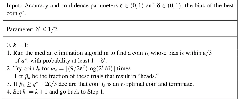
Suppose we are given a vector q∈[0,1]n, and we are told that the true vector p of coin biases is a permutation of q. The policy in Table 1 takes as input the accuracyε, the confidence parameterδ, and the vector q. In fact the policy only needs to know the bias of the best coin, which we denote by q∗=max`q`. The policy also uses an additional parameterδ0∈(0,1/2].
The following theorem establishes the correctness of the policy, and provides an upper bound on the expected number of trials.
Theorem 11 For everyδ0∈(0,1/2],ε∈(0,1), andδ∈(0,1), the policy in Table 1 is guaranteed to terminate after a finite number of steps, with probability 1, and is (q,ε,δ)-correct. For every permutationσ, the expected number of trials satisfies
Eq◦σ[T]≤ 1
ε2
c1n+c2log 1
δ
,
for some positive constants c1and c2that depend only onδ0.
Proof We start with a useful calculation. Suppose that at iteration k, the median elimination algo-rithm selects a coin Ikwhose true bias is pIk. Then, using the Hoeffding inequality, we have
P(|pˆk−pIk| ≥ε/3)≤exp{−2(ε/3) 2m
k} ≤
δ
Input: Accuracy and confidence parameters ε∈(0,1) andδ∈(0,1); the bias of the best coin q∗.
Parameter:δ0≤1/2.
0. k=1;
1. Run the median elimination algorithm to find a coin Ikwhose bias is withinε/3 of q∗, with probability at least 1−δ0.
2. Try coin Ik for mk=d(9/2ε2)log(2k/δ)etimes.
Let ˆpkbe the fraction of these trials that result in “heads.”
3. If ˆpk≥q∗−2ε/3 declare that coin Ikis anε-optimal coin and terminate. 4. Set k :=k+1 and go back to Step 1.
Table 1: A policy for finding anε-optimal coin when the bias of the best coin is known.
Let K be the number of iterations until the policy terminates. Given that K >k−1 (i.e., the policy did not terminate in the first k−1 iterations), there is probability at least 1−δ0≥1/2 that
pIk ≥q∗−(ε/3), in which case, from Eq. (18), there is probability at least 1−(δ/2
k)≥1/2 that
ˆ
pk≥q∗−(2ε/3). Thus, P(K>k|K>k−1)≤1−η, withη=1/4. Consequently, the probability that the policy does not terminate by the kth iteration, P(K>k), is bounded by(1−η)k. Thus, the probability that the policy never terminates is bounded above by(3/4)kfor all k, and is therefore 0. We now bound the expected number of trials. Let c be such that the number of trials in one execution of the median elimination algorithm is bounded by(cn/ε2)log(1/δ0). Then, the number of trials, t(k), during the kth iteration is bounded by (cn/ε2)log(1/δ0) +mk. It follows that the
expected total number of trials under our policy is bounded by
∞
∑
k=1
P(K≥k)t(k) ≤ 1
ε2
∞
∑
k=1
(1−η)k−1cn log(1/δ0) + (9/2)log(2k/δ) +1
= 1
ε2
∞
∑
k=1
(1−η)k−1 cn log(1/δ0) + (9/2)log(1/δ) + (9k/2)log 2+1
≤ ε12(c1n+c2log(1/δ)), for some positive constants c1and c2.
We finally argue that the policy is (q,ε,δ)-correct. For the policy to select a coin I with bias
pI ≤q∗−ε, it must be that at some iteration k, a coin Ik with pIk ≤q∗−ε was obtained, but ˆpk
came out larger than q∗−2ε/3. From Eq. (18), for any fixed k, the probability of this occurring is bounded byδ/2k. By the union bound, the probability that pI≤q∗−εis bounded by∑∞k=1δ/2k=δ.
considered in the proofs of Theorems 1 and 5: under those hypotheses, the value of q∗is not a priori known. We note that Theorem 11 disagrees with a lower bound in a preliminary version (Mannor and Tsitsiklis, 2003) of this paper. It turns out that the latter lower bound is only valid under an additional restriction on the set of policies, which will be the subject of Section 7.3.
7.2 A Lower Bound
We now prove that the upper bound in Theorem 11 is tight, within a constant.
Theorem 13 There exist positive constants c1, c2, ε0, and δ1, such that for every n≥2 andε∈
(0,ε0), there exists some q∈[0,1]n, such that for everyδ∈(0,δ1)and every (q,ε,δ)-correct policy,
there exists some permutationσsuch that
Eq◦σ[T]≥ ε12
c1n+c2log 1
δ
.
Proof Letε0=1/4 and letδ1=δ0/5, where δ0is the same constant as in Theorem 5. Let us fix some n≥2 andε∈(0,ε0). We will establish the claimed lower bound for
q= (0.5+ε,0.5−ε, . . . ,0.5−ε), (19)
and for everyδ∈(0,δ1). In fact, it is sufficient to establish a lower bound of the form(c2/ε2)log(1/δ) and a lower bound of the form c1n/ε2. We start with the former.
Part I. Let us consider the following three hypothesis testing problems. For each problem, we are interested in a δ-correct policy, i.e., a policy whose probability of error is less thanδ under any hypothesis. We will show that aδ-correct policy for the first problem can be used to construct a
δ-correct policy for the third problem, with the same sample complexity, and then apply Theorem 5 to obtain a lower bound.
Π1: We have two coins and the bias vector is either(0.5−ε, 0.5+ε)or(0.5+ε, 0.5−ε). We wish to determine the best coin. This is a special case of our permutation problem, with n=2.
Π2: We have a single coin whose bias is either 0.5−εor 0.5+ε, and we wish to determine the bias of the coin.4
Π3: We have two coins and the bias vector can be(0.5,0.5−ε),(0.5+ε,0.5−ε), or(0.5,0.5+ε). We wish to determine the best coin.
Consider a δ-correct policy for problemΠ1 except that the coin outcomes are encoded as fol-lows. Whenever coin 1 is tried, record the outcome unchanged; whenever coin 2 is tried, record the opposite of the outcome (i.e., record a 0 outcome as a 1, and vice versa). Under the first hypothesis in problemΠ1, every trial (no matter which coin was tried) has probability 0.5−εof being equal to 1, and under the second hypothesis has probability 0.5+εof being equal to 1. With this encoding, it is apparent that the information provided by a trial of either coin in problemΠ1is the same as the
information provided by a trial of the single coin in problem Π2. Thus, a δ-correct policy forΠ1 translates to aδ-correct policy forΠ2, with the same sample complexity.
In problem Π3, note that coin 2 is the best coin if and only if its bias is equal to 0.5+ε(as opposed to 0.5−ε). Thus, anyδ-correct policy forΠ2 can be applied to the second coin inΠ3, to yield aδ-correct policy forΠ3with the same sample complexity.
We now observe that problemΠ3involves a set of three hypotheses, of the form considered in the proof of Theorem 5, for the case of two coins. More specifically, in terms of the notation used in that proof, we have p= (0.5,0.5−ε), and N(p,ε) ={2}. It follows that the sample complexity of anyδ-correct policy forΠ3 is lower bounded by(c1/ε2)log(1/8δ), where c1 is the constant in Theorem 5.5 Because of the relation between the three problems established earlier, the same lower bound applies to anyδ-correct policy for problemΠ1, which is the permutation problem of interest. We have so far established a lower bound proportional to (1/ε2)/log(1/δ) for problemΠ
1, which is the permutation problem we are interested in, with a q vector of the form (19), for the case
n=2. Consider now the permutation problem for the q vector in (19), but for general n. If we are given the information that the best coin can only be one of the first two coins, we obtain problem
Π1. In the absence of this side-information, the permutation problem cannot be any easier. This shows that the same lower bound holds for every n≥2.
Part II: We now continue with the second part of the proof. We will establish a lower bound of the form c1n/ε2 for the permutation problem associated with the bias vector q introduced in Eq. (19), to be referred to as problemΠ. The proof involves a reduction of Πto a problem ˜Πof the form considered in the proof of Theorem 5.
The problem ˜Πinvolves n+1 coins (coins 0,1, . . . ,n)and the following n+2 hypotheses:
H00 : p0=0.5, pi=0.5−ε,for i6=0,
H000: p0=0.5+ε, pi=0.5−ε, for i6=0, and
H`: p0=0.5, p`=0.5+ε, pi=0.5−ε,for i6=0, `.
Note that the best coin is coin 0 under either hypothesis H00 or H000, and the best coin is coin`under
H`, for`≥1. This leads us to define H0as the hypothesis that either H00 or H000is true.
We say that a policy for ˜Πisδ-correct if it selects the best coin with probability at least 1−δ. We will show that if we have a(q,ε,δ)-correct policyπforΠ, with a certain sample complexity, we can construct an(ε,5δ)-correct policy ˜πwith a related sample complexity. We will then apply Theorem 5 to lower bound the sample complexity of ˜π, and finally translate to a lower bound forπ. The idea of the reduction is as follows. In problem ˜Π, if we knew that H0is not true, we would be left with a permutation problem with n coins, to whichπcould be applied. However, if H0 is true, the behavior ofπis unpredictable. (In particular,πmight not terminate, or it might terminate with an arbitrary decision: this is because we are only assuming thatπbehaves properly when faced with the permutation problem Π.) If H0 is true, we can replace coin 1 with a coin whose bias is 0.5+ε, resulting in the bias vector q, in which caseπis guaranteed to work properly. But what if we replace coin 1 as above, but some H`,`6=0,1, happens to be true? In that case, there will be two
coins with bias 0.5+εandπmay misbehave. The solution is to run two processes in parallel, one
with and one without this modification, in which case one of the two will have certain performance guarantees that we can exploit.
Consider the(q,ε,δ)-correct policyπfor problemΠ. Let tπbe the maximum (over all permuta-tionsσ) expected time untilπterminates when the true coin bias vector is q◦σ.
We define two more bias vectors that will be used below:
q−= (0.5−ε, . . . ,0.5−ε),
and
q+= (0.5+ε, 0.5+ε,0.5−ε, . . . ,0.5−ε).
Note that if H0is true in problem ˜Π, andπis applied to coins 1, . . . ,n, thenπwill be faced with the bias vector q−. Also, if H`, is true in problem ˜Π, for some`6=0,1, and we modify the bias of coin
1 to 0.5+ε, then policyπwill be faced with the bias vector q+.
Let us note for future reference that, as in Eq. (18), if we sample a coin with bias 0.5+εfor
m=4d(1/ε2)log(1/δ)etimes, the empirical mean reward is larger than 0.5 with probability at least 1−δ. Similarly, if we sample a coin with bias 0.5−ε for m times, the empirical mean reward is smaller than 0.5 with probability at least 1−δ. Sampling a specific coin that many times, and comparing the empirical mean to 0.5, will be referred to as “validating” the coin.
We now describe policy ˜πfor problem ˜Π. The policy involves two parallel processes
A
andB
: it alternates between the two processes, and each process samples one coin in each one of its turns. The processes continue to sample the coins alternately until one of them terminates and declares one of the coins as the best coin (or equivalently selects a hypothesis). The parameter k below is set to k=d18 log(1/δ)e.A
: Apply policy π to coins 1,2, . . . ,n. If π terminates and selects coin `, validate coin ` by sampling it m times. If the empirical mean reward is more than 0.5, thenA
terminates and declares coin`as the best coin. If the empirical mean reward is less than or equal to 0.5, thenA
terminates and declares coin 0 as the best coin. Ifπhas carried outdtπ/δetrials, thenA
terminates and declares coin 0 as the best coin.B
: Sample coin 1 for m times. If the empirical mean reward is more than 0.5, thenB
terminates and declares coin 1 as the best coin. Otherwise, replace coin 1 with another coin whose bias is 0.5+ε. Initialize a counter N with N=0.Repeat k times the following:
(a) Pick a random permutationτ(uniformly over the set of permutations).
(b) Run aτ-permuted version ofπ, to be referred to asτ◦π; that is, wheneverπis supposed to sample coin i,τ◦πsamples coinτ(i)instead.
(c) Ifτ◦πterminates and selects coin 1 as the best coin, set N :=N+1.
If N>2k/3, then
B
terminates and declares coin 0 as the best coin. Otherwise, wait until processA
terminates.1. Process
A
terminates first, H0is true. In this case the true bias vector faced byπis q−ratherthan q. An error can happen only ifπterminates and the coin erroneously passes the validation test. The probability of this occurring is at mostδ. In all other cases (validation fails or the running time exceeds the time limitdtπ/δe), process
A
correctly declares H0 to be the true hypothesis.2. Process
A
terminates first, H`is true for some`6=0. ProcessA
does not declare the correctH` if one of the following events occurs:
A
fails to select the best coin (probability at mostδ, sinceπis(q,ε,δ)-correct); or the validation makes an error (probability at mostδ); or the time limit is exceeded. By Markov’s inequality, the probability that the running time Tπof policyπexceeds the time limit satisfies
Pq(Tπ≥tπ/δ)≤Eq[Tπ]δ/tπ≤tπδ/tπ=δ.
So, the total the probability of errors that fall within this case is bounded by 3δ.
3. Process
B
terminates first, H0 is true. Note that under H0, processB
is faced with n coins whose bias vector is q. ProcessB
does not declare H0if one of the following events occurs: the initial validation of coin 1 makes an error (probability at mostδ); or in k runs, the permuted versions of policy πmake at least k/3 errors. Each such run has probability at mostδ of making an error (sinceπis(q,ε,δ)-correct), independently for each run (because we use a random permutation before each run). Using Hoeffding’s inequality, the probability of at leastk/3 errors is bounded by exp{−2k(1/3−δ)2}. Sinceδ<1/12, this probability is at most
e−k/8. So, the total the probability of errors that fall within this case is bounded byδ+e−k/8. 4. Process
B
terminates first, H`is true for some` >1. ProcessB
does not declare H`if oneof the following events occurs: the initial validation of coin 1 makes an error (probability at mostδ); or in k runs, the permuted versions of policy πselect coin 1 for N >2k/3 times. Since in each of the k runs the policy is faced with the bias vector q+, there are no guarantees
on its behavior. However, since we use a random permutation before each run, and since there are two coins with bias 0.5+ε, namely coins 1 and`, the probability that the permuted version ofπselects coin 1 at any given run is bounded by 1/2. Using Hoeffding’s inequality, the probability of selecting coin 1 more than 2k/3 times is bounded by exp{−2k((2/3)− (1/2))2}=e−k/18. So, the total the probability of errors that fall within this case is bounded byδ+e−k/18.
5. Process
B
terminates first, H1is true. ProcessB
fails to declare coin 1 only if an error is made in the initial validation step, which happens with probability bounded byδ.To conclude, using the union bound, when H0 is true, the probability of error is bounded by 2δ+e−k/8 ; when H
1 is true, it is bounded by 4δ; and when H`, ` >1 is true, it is bounded by
4δ+e−k/18. Since k=18 log(1/δ), we see that the probability of error, under any hypothesis, is bounded by 5δ.
We now examine the sample complexity of policy ˜π. We consider two cases, depending on which hypothesis is true.
1. H0 is true. In process