Fusion of Domain Knowledge with Data for Structural Learning in
Object Oriented Domains
Helge Langseth∗ [email protected]
Thomas D. Nielsen [email protected]
Department of Computer Science, Aalborg University Fredrik Bajers Vej 7E, DK-9220 Aalborg Ø, Denmark
Editors: Richard Dybowski, Kathryn B. Laskey, James W. Myers and Simon Parsons
Abstract
When constructing a Bayesian network, it can be advantageous to employ structural learning algo-rithms to combine knowledge captured in databases with prior information provided by domain ex-perts. Unfortunately, conventional learning algorithms do not easily incorporate prior information, if this information is too vague to be encoded as properties that are local to families of variables. For instance, conventional algorithms do not exploit prior information about repetitive structures, which are often found in object oriented domains such as computer networks, large pedigrees and genetic analysis.
In this paper we propose a method for doing structural learning in object oriented domains. It is demonstrated that this method is more efficient than conventional algorithms in such domains, and it is argued that the method supports a natural approach for expressing and incorporating prior information provided by domain experts.
Keywords: Bayesian networks, structural learning, object orientation, knowledge fusion
1. Introduction
The Bayesian network (BN) framework (Pearl, 1988; Jensen, 1996, 2001) has established itself as a powerful tool in many areas of artificial intelligence. However, eliciting a BN from a domain expert can be a laborious and time consuming process. Thus, methods for learning the structure of a BN from data have received much attention during the last years. For an overview see Buntine (1996) and Krause (1998). Current learning methods have been successfully applied in learning the structure of BNs based on databases. Unfortunately, though, only to a small extent do these methods incorporate prior information provided by domain experts. Prior information is typically encoded by specifying a prior BN hence, this information is restricted to the occurrence/absence of edges between specific pairs of variables.
In domains that can appropriately be described using an object oriented language (Mahoney and Laskey, 1996; Mathiasen et al., 2000) we typically find repetitive substructures or substructures that can naturally be ordered in a superclass–subclass hierarchy. For such domains, the expert is usually able to provide information about these properties. However, this information is not easily exploited by current learning methods due to the practice mentioned above.
Recently, object oriented versions of the BN framework (termed OOBNs) have been proposed in the literature, see for example Mahoney and Laskey (1996), Laskey and Mahoney (1997), Koller and Pfeffer (1997), and Bangsø and Wuillemin (2000b). Although these object oriented frameworks relieve some of the problems when modelling large domains, it may still prove difficult to elicit the parameters and the structure of the model. Langseth and Bangsø (2001) describe a method to efficiently learn the parameters in an object oriented domain model, but the problem of specifying the structure still remains.
In this paper we propose a method for doing structural learning in an object oriented domain based on the OOBN framework. We argue that OOBNs supply a natural framework for encoding prior information about the general structure of the domain. Moreover, we show how this type of prior information can be exploited during structural learning. Empirical results demonstrate that the proposed learning algorithm is more efficient than conventional learning algorithms in object oriented domains.
2. Object Oriented Bayesian Networks
Using small and “easy-to-read” pieces as building blocks to create a complex model is an often applied technique when constructing large Bayesian networks. For instance, Pradhan et al. (1994) introduce the concept of sub-networks, which can be viewed and edited separately, and frameworks for modelling object oriented domains have been proposed by Mahoney and Laskey (1996), Laskey and Mahoney (1997), Koller and Pfeffer (1997), and Bangsø and Wuillemin (2000b).
In what follows the framework of Bangsø and Wuillemin (2000b) will be described, as it forms the formal basis for the proposed learning method. Note that we limit the description to those parts of the framework that are relevant for the learning algorithm. Further details can be found in the papers by Bangsø and Wuillemin (2000a,b).
2.1 The OOBN Framework
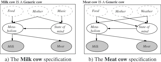
Consider a farm with two milk cows and two meat cows, and assume that we are interested in modelling the environment’s effect on the milk and meat production of these cows.1 Following the object oriented idea (Mathiasen et al., 2000), we construct a Generic cow class that describes the general properties common to all cows (see Figure 1): Specifically, as we are interested in the milk and meat production, we let Milk and Meat be output nodes of the class (depicted by shaded ellipses). That is to say, nodes from a class usable outside the instantiations of the class. Assuming that both the mother of a cow and the food a cow eats influence its milk and meat production, we let Mother and Food be input nodes (depicted by dashed ellipses) of the class; an input node is a reference to a node defined outside the scope of the instantiations of the class. Nodes that are neither input nodes nor output nodes are termed normal nodes. Note that the input nodes and output nodes form the interface between an instantiation and the context in which the instantiation exists. In the remainder of this paper we assume that all nodes are discrete.
A class may be instantiated several times with different nodes having influence on the different instantiations through the input nodes hence, only the state space (the states and their ordering) of the input nodes is known at the time of specification2(for example, the cows might have different
moth-1. A milk cow primarily produces milk and a meat cow primarily produces meat.
ers). To avoid ambiguity when referring to a node in a specific instantiation, the name of the node will sometimes be prefixed by the name of the instantiation (that is, INSTANTIATION-NAME. Node-name).
Food
bolism Meta-Mother
Milk Meat
Generic cow
Figure 1: General properties common to all cows are described using the class Generic cow. The arrows are links as in normal BNs. The dashed ellipses are input nodes, and the shaded ellipses are output nodes.
In order to model the different properties of milk cows and meat cows, we introduce the two classes Milk cow and Meat cow (see Figure 2). These two cow specifications are subclasses of the Generic cow class (hence the “IS A Generic cow” in the top left corner of each of the class specifications). In a general setting, a class S can be a subclass of another class C if S contains at least the same set of nodes as C. This ensures that an instantiation of S can be used anywhere in the OOBN instead of an instantiation of C (e.g., an instantiation of Milk cow can be used instead of an instantiation of Generic cow). Each node in a subclass inherits the conditional probability table (CPT) of the corresponding node in its superclass unless the parent sets differ, or the modeler explicitly overwrites the CPT. The sub–superclass relation is transitive but not anti-symmetric, so to avoid cycles in the class hierarchy it is required that a subclass of a class cannot be a superclass of that class as well. Furthermore, multiple inheritance is not allowed, so the structure of the class hierarchy will be a tree or a collection of disjoint trees (called a forest).
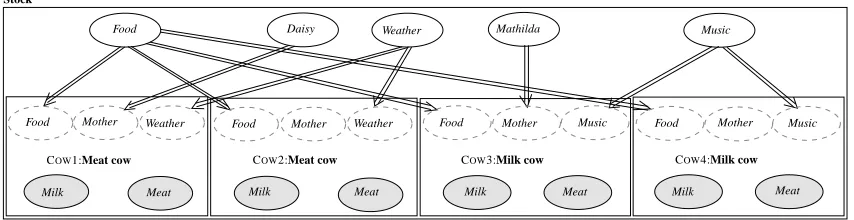
Finally, to model the four cows in the live-stock we construct a class Stock that encapsulates the corresponding instantiations. In Figure 3 the boxes represent instantiations. For example, COW1 is
Food
Meta-mind Music
bolism
State of Mother
Milk cow IS A Generic cow
Meat Milk
Mother
mind State of
Weather
Meta-bolism
Food
Meat cow IS A Generic cow
Meat Milk
a) The Milk cow specification b) The Meat cow specification
an instantiation of the class Meat cow, which is indicated by COW1:Meat cow inside the COW1 instantiation. Note that only input nodes and output nodes are visible, as they are the only part of an instantiation which directly interact with the encapsulating context (in this case the Stock class). This does not impose any constraints on which variables may be observed, it is merely a design technique to easier maintain large domain models. The double arrows are reference links. A reference link indicates that the leaf of the link is a reference (or pointer) to the root of that link.3 For instance, the input node Mother of COW1 is a reference to the node Daisy. This means that whenever the node Mother is used inside the instantiation COW1, the node Daisy will be the node actually used (for instance during inference).
Mathilda Weather
Food
COW1:Meat cow Food Mother Weather
COW3:Milk cow Food
Mother Mother
COW4:Milk cow Music Food Mother
Food Weather Music
Music Daisy
Stock
COW2:Meat cow
Meat
Milk Milk Meat Milk Meat Milk Meat
Figure 3: The Stock class with two instantiations of the Milk cow class and two instantiations of the Meat cow class. Note that some input nodes are not referencing any nodes.
If there is more than one instantiation of a class (for example, COW1 and COW2 in Figure 3), the OOBN framework gives rise to the OO assumption (Langseth and Bangsø, 2001). This assumption states that the CPTs of one instantiation of a class are identical to the corresponding CPTs of any other instantiation of that class (meaning that the domains of the CPTs are compatible and that the table entries are identical).
As the subclasses in a class hierarchy may have a larger set of nodes than their superclasses, the input set of a subclass S might be larger than the input set of its superclass C. Thus, if an instantiation of S is used instead of an instantiation of C, the extra input nodes will not be referencing any nodes. To ensure that these nodes are associated with potentials, the notion of a default potential is introduced: A default potential is a probability distribution over the states of an input node that is used when the input node is not referencing any node. Note that a default potential can also be used when no reference link is specified, even if this is not a consequence of subclassing. As an example we have that not all the Mother nodes in Figure 3 reference a node, but because of the default potential all nodes are still associated with a CPT. It is also worth noticing that the structure of references is always a tree or a forest; cycles of reference links are not possible (Bangsø and Wuillemin, 2000a).
Finally, inference can be performed by translating the OOBN into a multiply-sectioned Bayesian network (Xiang et al., 1993; Xiang and Jensen, 1999), see Bangsø and Wuillemin (2000a) for details on this translation. Alternatively, we can construct the underlying BN of the OOBN: The underlying
BN of an instantiation I, BNI, is the (conventional) BN that corresponds to I including all encapsu-lated instantiations. There is exactly one such underlying BN for a given instantiation, and it can be constructed using the following algorithm (Langseth and Bangsø, 2001):
Algorithm 1 (Underlying BN)
1. Let BNIbe the empty graph.
2. Add a node to BNIfor all input nodes, output nodes and normal nodes in I.
3. Add a node to BNIfor each input node, output node and normal node of the instantiations
en-capsulated in I, and prefix the name of the instantiation to the node name (INSTANTIATION-NAME .Node-name). Do the same for instantiations contained in these instantiations, and so on.
4. Add a link for each normal link in I, and repeat this for all instantiations as above.
5. For each reference tree, merge all the nodes into one node. This node is given all the parents and children (according to the normal links) of the nodes in the reference tree as its family. Note that only the root of the tree can have parents, as all other nodes are references to this node.
An input node that does not reference another node will become a normal node equipped with a default potential. This can also be seen in Figure 4 which depicts the underlying BN of an instanti-ation of the Stock-class (Figure 3).
COW4.
mind State of
COW1. COW2. COW3. COW4.
Mother
COW4. COW2.
Meat Milk Milk Milk
Milk
COW1. COW1.
Meat
COW2. COW3.
COW2. COW3.
Meat
Mother Weather
State of Food
Daisy Mathilda Music
COW4. COW4.
Meat Metabolism
COW1.
mind Metabolism Metabolism Metabolism State of
COW2.
mind
State of C
OW3.
mind
Figure 4: The underlying BN for the OOBN depicted in Figure 3.
Note that nodes associated with default potentials (COW2.Mother and COW4.Mother) can be marginalized out as they have no effect in the underlying BN. It is also worth emphasizing that an OOBN is just a compact representation of a (unique) BN that satisfies the OO assumption, namely the underlying BN (this can also immediately be seen from Algorithm 1).
2.2 The Insurance Network
SocioEcon
GoodStudent RiskAversion
VehicleYear MakeModel AntiTheft HomeBase
OtherCar Age
DrivingSkill SeniorTrain
MedCost
DrivQuality DrivHist RuggedAuto Antilock
CarValue Airbag
Accident
ThisCarDam OtherCarCost ILiCost
ThisCarCost
Cushioning Mileage
PropCost Theft
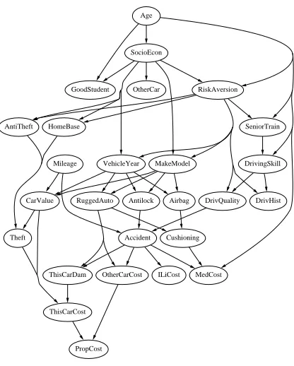
Figure 5: The insurance network, used for classifying car insurance applications.
The corresponding OOBN representation of this network is based on six classes (Insurance,
Theft, Accident, Car, Car owner and Driver), which can be seen as describing different (abstract)
entities in the domain. These classes are designed such that they adhere to the design principle of high internal coupling and low external coupling, see for example Mahoney and Laskey (1996) and Mathiasen et al. (2000).
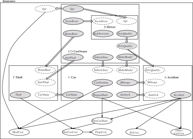
For instance, the class Car describes the properties associated with a car (specific for this do-main). The nodes Cushioning, Mileage, CarValue, RuggedAuto and Antilock are the only nodes “used” outside the class hence, they occur as output nodes whereas Vehicle year and Make model are input nodes and Airbag is a normal node (see also the encapsulated instantiation C:Car in Fig-ure 2.2). As another example, consider the class Driver, which models the driving characteristics of a car owner. In the insurance context, driving characteristics are an integral part of the notion of a car owner and (by the above mentioned design principle) an instantiation of Driver is therefore encapsulated in the class CarOwner. The class Insurance encapsulates the corresponding instan-tiations of the other classes. Figure 2.2 depicts the final OOBN model in form of the Insurance class. Note that only the interfaces of the encapsulated instantiations are shown.
ThisCarDam
CarCost Other-D:Driver
Insurance
C:Car T:Theft
CO:CarOwner
SocioEcon SocioEcon Age
HomeBase
AntiTheft
DrivQuality
DrivQuality
MakeModel VehicleYear
RiskAversion
Mileage
A:Accident
Accident CarValue
Mileage Cushioning
DrivQuality
Antilock Antilock
VehicleYear MakeModel Age
Age
HomeBase
AntiTheft
CarValue Theft
MedCost ThisCarCost PropCost RuggedAuto
ILiCost
Figure 6: An OOBN representation of the insurance network. Notice that only the interfaces of the encapsulated instantiations are shown. Note also that we use a slightly non-standard graphical presentation for visualization purposes.
That is, T.CarValue is a reference to C.CarValue. This is required since CarValue is defined outside the scope of the instantiations of the Theft-class.
2.3 OOBNs and Dynamic Bayesian Networks
An important set of Bayesian networks is dynamic Bayesian networks (DBNs), which model the stochastic evolution of a set of random variables over time, see for example Kjærulff (1992). Tra-ditionally, a DBN specification consists of i)a BN over the variables at t=0, and ii) a transition BN over the variables at t=0 and t=1. These two networks can alternatively be described using OOBN classes, where the time-dependence is encoded by references between nodes; a self-reference is a self-reference between a node and an input node in the same class.4 More precisely, when using the OOBN framework for modelling DBNs we construct two classes: One class represent-ing the time-slice at t=0, and another class whose instantiations correspond to the time-slices at t>0. The dependence relation between a time-slice and the previous time-slice is then represented using self-references within the class specification, see also Bangsø and Wuillemin (2000b). Note that using OOBN classes for modelling time-slices also supports the introduction of encapsulated instantiations within the time slices.
3. Structural Learning
In what follows we review the basis for performing structural learning. The notation will, whenever possible, follow that of Cooper and Herskovits (1991) and Heckerman et al. (1995).
Consider a Bayesian network BN= (BS,ΘBS)over a set of discrete variables {X1,X2, ...,Xn},
where BS is the graphical structure and ΘBS is the quantitative information. To describe BS, the
qualitative aspects of BN, we will use the following notation: ri is the number of states for variable
Xi, qi=∏Xl∈Πirl is the number of configurations over the parents for Xiin BS(denoted byΠi), and
Πi=j denotes the event thatΠi takes on its j’th configuration. For the quantitative properties, we
useθi jk=P(Xi=k|Πi= j,ξ) (we assumeθi jk >0), whereξis the prior knowledge. For ease of
exposition we define
Θi j =∪rki=1θi jk; Θi=∪qji=1Θi j; ΘBS=∪
n i=1Θi.
Note that ∀i,j :∑ri
k=1θi jk=1. Finally, we let
D
={D1,...,DN} denote a database of N cases,where each case is a configuration x over the variables X= (X1,...,Xn).
The task is now to find a structure BSthat best describes the observed data, or in a more abstract
formulation, to find the parameter spaceΩBS that best restricts the parameters used to describe the
family of probability distributions
F
ΩBS ={f(x|Θ):Θ∈ΩBS}. For example, letΩ0be theparam-eter space required to describe all probability distributions compatible with the complete graph for two binary variables X1 and X2 (see Figure 7a). With the above notation, Ω0 is defined so that
(θ1,θ21,θ22)∈Ω0. For the empty graph in Figure 7b, the parameter spaceΩ00⊂Ω0 corresponds to the parameter spaceΩ0whereθ21=θ22hence,Ω00is a hyperplane inΩ0. Learning the structure BS
is therefore equivalent to finding the parameter spaceΩBS that best describes the data; when
learn-ing the structure of a BN there is an injective mapplearn-ing from the BN structure, BS, to the associated
parameter space ΩBS. However, as we shall see in Section 5, when we focus on learning OOBNs
this is no longer true as some aspects (the OO-assumption) of an OOBN are not reflected in the underlying graphical structure. In that case it may be beneficial to think of structural learning as learning a parameter spaceΩ.
X1 X2 X1 X2
a) Complete graph b) Empty graph
Figure 7: The two BN model structures for the domain X= (X1,X2).
3.1 The BD Metric
A Bayesian approach for measuring the quality of a BN structure BS, is its posterior probability
given the database:
P(BS|
D
,ξ) =c·P(BS|ξ)P(D
|BS,ξ),where c=1/(∑BP(B|ξ)P(
D
|B,ξ)). The normalization constant c does not depend on BS, thusP(
D
,BS|ξ) =P(BS|ξ)P(D
|BS,ξ)is usually used as the network score. Note that the maincompu-tational problem is the calculation of the marginal likelihood:
P(
D
|BS,ξ) =Z
ΘBS
since the integral is over all possible parameters (conditional probabilities) ΘBS hence, over all
possible BNs that encode at least the same conditional independence relations as the structure BS.
Cooper and Herskovits (1991) showed that this probability can be computed in closed form based on the following five assumptions:
1. The database
D
is a multinomial sample from some Bayesian network BGwith parametersΘBG.
2. the cases in the database
D
are independent given the BN model.3. The database is complete, that is, there does not exist a case in
D
with missing values.4. For any two configurations over the parents for a variable Xi, the parameters for the
condi-tional probability distributions associated with Xiare marginally independent (Θi j⊥⊥Θi j0 for
j6= j0).
5. The prior distribution of the parameters in every Bayesian network BShas a Dirichlet
distri-bution.5 That is to say, there exist numbers (virtual counts) Ni jk0 >0 such that
P(Θi j|BS,ξ) =
Γ(∑ri
k=1Ni jk0 )
∏ri
k=1Γ(Ni jk0 ) ri
∏
k=1
θNi jk0 −1
i jk , (2)
whereΓis the Gamma function satisfyingΓ(x+1) =xΓ(x). Note that the virtual counts can be seen as pseudo counts similar to the sufficient statistics derived from the database.
An implicit assumption by Cooper and Herskovits (1991) is parameter modularity: The densities of the parametersΘi jdepend only on the structure of the BN that is local to variable Xi.
Now, let Ni jkbe the sufficient statistics given by Ni jk=∑Nl=1γ(Xi=k,Πi=j : Dl), whereγ(Xi=
k,Πi = j : Dl) takes on the value 1 if(Xi=k,Πi = j) occurs in case Dl, and 0 otherwise. From
Assumptions 1, 2 and 3 we then have
P(
D
|BS,ΘBS,ξ) =n
∏
i=1
qi
∏
j=1
ri
∏
k=1
θNi jk
i jk . (3)
Substituting Equation 3 into Equation 1 gives
P(
D
|BS,ξ) =Z
ΘBS
n
∏
i=1
qi
∏
j=1
ri
∏
k=1
θNi jk
i jk P(ΘBS|BS,ξ)dΘBS,
and by Assumptions 4 and 5 we get
P(
D
|BS,ξ) = n∏
i=1
qi
∏
j=1
Z
Θi j
ri
∏
k=1
θNi jk
i jk
"
Γ(∑ri
k=1Ni jk0 )
∏ri
k=1Γ(Ni jk0 ) ri
∏
k=1
θNi jk0 −1
i jk
# dΘi j
=
∏
ni=1
qi
∏
j=1
Γ(∑ri
k=1Ni jk0 )
∏ri
k=1Γ(Ni jk0 )
Z
Θi j
ri
∏
k=1
θNi jk+Ni jk0 −1
i jk dΘi j.
The expression ∏ri
k=1θ
Ni jk+Ni jk0 −1
i jk corresponds to the last term of the Dirichlet distribution for the
parametersΘi jhaving counts Ni jk+Ni jk0 . Since this is a probability distribution over the parameters,
the value of the integral can be read directly from Equation 2 (the integral over all parameters evaluates to 1) and we get
P(
D
,BS|ξ) =P(BS|ξ) n∏
i=1
qi
∏
j=1
Γ(Ni j0)
Γ(Ni j+Ni j0) ri
∏
k=1
Γ(Ni jk+Ni jk0 )
Γ(Ni jk0 ) , (4)
where Ni j=∑rki=1Ni jkand Ni j0 =∑ ri
k=1Ni jk0 . This metric is known as the BD metric (Bayesian metric
with Dirichlet priors), and it was first derived by Cooper and Herskovits (1992). Unfortunately it requires the specification of the virtual counts Ni jk0 for all variable–parent configurations and for all values i, j and k.
3.2 The BDe Metric
One drawback of the BD metric is that networks, which are likelihood equivalent, need not be given the same score.6 Note that data cannot be used to discriminate between such networks. Another shortcoming of the BD metric is that it does not provide an easy way of specifying prior informa-tion concerning network structure and parameters. To overcome these problems, Heckerman et al. (1995) describe the BDe metric (Bayesian metric with Dirichlet priors and equivalence) that gives the same score to likelihood equivalent networks. Hence, the metric is based on the concept of sets of likelihood equivalent network structures, where all members in a set are given the same score.
The BDe metric also provides a simple way of identifying the virtual counts Ni jk0 (in Equation 4) by having the user specify a prior Bayesian network Bpfor X and an equivalent sample size N0:
Ni jk0 =P(Xi=k,Πi= j|Bp,ξ)·N0. (5)
Note that Heckerman et al. (1995) actually condition on a complete network BSc consistent with
Bp; conditioning on BSc allows Heckerman et al. (1995) to show that the Dirichlet assumption
(Assumption 5) is not required. Finally, to evaluate Equation 4 we also need to define a prior probability P(BS|ξ)for the network structures. Different prior probabilities have been proposed in
the literature, most of which obey the structural modularity assumption:
P(BS|ξ)∝ n
∏
i=1
ρ(Xi,Πi).
That is, the prior probability decomposes into a product with one term for each family in the net-work. From this assumption Equation 4 can be expressed as
P(
D
,BS|ξ)∝ n∏
i=1
ρ(Xi,Πi)·score(Xi,Πi,
D
),where
score(Xi,Πi,
D
) = qi∏
j=1
Γ(Ni j0)
Γ(Ni j+Ni j0) ri
∏
k=1
Γ(Ni jk+Ni jk0 )
Γ(Ni jk0 ) .
Hence, when comparing two network structures we only need to consider the (local) scores and priors for the families for which they differ.
3.3 Learning from Incomplete Data
In real world problems we rarely have access to a complete database hence, assumption 3 of the BD metric (and the BDe metric) is likely to be violated. This implies that the parameters for a model become dependent, and known closed-form expressions cannot be used to calculate the marginal likelihood of the data. In such situations, a common approach is to apply asymptotic approximations such as the Laplace approximation, (see, for example, Ripley, 1996), the Bayesian Information Criterion (Schwarz, 1978), the Minimum Description Length (Rissanen, 1987) or the Cheeseman-Stutz approximation (Cheeseman and Cheeseman-Stutz, 1996), see also Chichering and Heckerman (1997) for a discussion. These approximations assume that the posterior over the parameters is peaked, and the maximum a posteriori (MAP) parameters are used when approximating the integral in Equation 1. Thus, in order to apply these approximations we need to find the MAP parameters, for example by using the expectation-maximization (EM) algorithm (Dempster et al., 1977; Green, 1990), before we can calculate the score of a model. Thus, for each candidate model we may need to invest a considerable amount of time in order to evaluate the model.
As an alternative, Friedman (1998) describes the Structural EM (SEM) algorithm which basi-cally “fills in” the missing values before searching the joint space of network structures and pa-rameters (we therefore avoid the computational expensive step of calculating the MAP papa-rameters for each candidate model). The validity of the SEM algorithm is based on the assumption that the data is missing at random (Little and Rubin, 1987), which is also assumed in the remainder of this paper. Informally, this means that the pattern of missingness may only depend on the values of the observed variables.7
The SEM algorithm maximizes P(
D
,BS|ξ), but instead of maximizing this score directly itmaximizes the expected score. Let o be the set of observations from the database
D
, and let h be the set of unobserved entries inD
. The general algorithm can then be outlined as:Algorithm 2 (SEM)
Loop for n=0,1,...until convergence
1) Compute the posterior P(ΘBn S|B
n S,o).
2) E-step: For each BS, compute:
Q(BS: BnS) = Eh[log P(h,o,BS)|BnS,o]
=
∑
h
P(h|o,BnS)log P(h,o,BS).
3) M-step: Choose BnS+1←BSthat maximizes Q(BS: BnS).
4) If Q(BnS: BnS) =Q(BnS+1: BnS)then Return BnS.
In the E-step, the algorithm completes the database by “filling-in” the unobserved entries based on the observations o, the current best model BnS, and the posterior over the parameters for BnS (calculated in step 1). From the completed database the best candidate model is then selected in the
the expected score at each iteration we always obtain a better network in terms of its marginal score (this result also implies that the algorithm converges).
By exploiting linearity of expectation in the E-step, Friedman (1998) shows that the expected score decomposes as if the data were complete. That is, local changes to the model does not require that the entire model is reevaluated. In our context this yields (for notational convenience we assume that the structural prior,∏ni=1ρ(Xi,Πi), is normalized):
Eh[log P(h,o,BS)|BnS,o] = n
∑
i=1
Eh[log Fi(Ni··(h,o),BS)|BnS,o], (6)
where Ni··(h,o)specifies the collection Ni jkaccording to(h,o), for all j and k, and Fi(Ni··(h,o),BS) =
ρ(Xi,Πi)score(Xi,Πi,h,o). Note that if∏ni=1ρ(Xi,Πi)is not normalized we simply subtract log(c),
where c is the normalization constant. That is to say, normalization of the prior distribution is not required. Friedman (1998) also examines an approximation forEh[log Fi(Ni··(h,o),BS)|BnS,o]:
Eh[log Fi(Ni··(h,o),BS)|BnS,o]≈log Fi(Eh[Ni··(h,o)|BnS,o],BS). (7)
The approximation is exact if log Fi is linear in its arguments. This is, however, not the case when
using the BD or BDe metric.8 Finally, the termEh[Ni··(h,o)|BnS,o]can be computed as
∀j,k :Eh[Ni jk(h,o)|BnS,o] = N
∑
l=1
P(Xi=k,Πi= j|Dl,BnS).
3.4 Learning Dynamic Bayesian Networks
Friedman et al. (1998) describe an algorithm for learning DBNs from both complete and incomplete data. The methods proposed by Friedman et al. (1998) extend both the Bayesian Information Crite-rion (BIC) and the BDe score for learning DBNs from complete data. When lifting the assumption that the database is complete, Friedman et al. (1998) extend the SEM algorithm accordingly.
Friedman et al. (1998) define a DBN by partitioning the variables into time-slices s.t. the vari-ables which occur at time t are denoted X[t]. Thus, a DBN with l time-slices consists of the variables X[0]∪X[1]∪···∪X[l]. It is assumed that the DBN is Markovian that is, P(X[t+1]|X[0],...,X[t]) = P(X[t+1]|X[t]). By also assuming that the DBN is stationary (the CPTs associated with the vari-ables in X[t]are independent of t, for t>0), a DBN can be completely described by two parts: i) An initial network, B0, that specifies a distribution over X[0]and ii)a transition network, B→, over the variables X[0]∪X[1].
In the context of DBNs, the database is assumed to consist of N cases, where the m’th case specifies a configuration over the variables X[0]∪X[1]∪ ··· ∪X[l]. Now, consider the situation where the database is complete and letθ0i j0k and θ→i jk be defined as in Section 3.1 for B0 and B→,
respectively; we use j0 and j to indicate that the parents for Xi may be different in B0 and B→.
Additionally, let the sufficient statistics be given by Ni j00k =∑Nm=1γ(Xi[0] =k,Πi = j0: Dm) and
Ni jk→ =∑lt=1∑Nm=1γ(Xi[t] =k,Πi= j : Dm). By derivations similar to those of the BD metric, the
following closed form expression for P(
D
,(B0,B→)|ξ)is obtained:P(
D
,(B0,B→)|ξ) = P((B0,B→)|ξ)·
∏
ni=1
q0i
∏
j0=1
Γ(Ni j000)
Γ(Ni j00+Ni j000)
ri
∏
k=1
Γ(Ni j00k+Ni j000k)
Γ(Ni j000k)
!
·
∏
ni=1
qi
∏
j=1
Γ(Ni j0→)
Γ(Ni j→+Ni j0→)
ri
∏
k=1
Γ(Ni jk→+Ni jk0→)
Γ(Ni jk0→) !
.
Note that when maximizing this expression we can consider the terms independently assuming that P(B0,B→|ξ) =P(B0|ξ)·P(B→|ξ).
Friedman et al. (1998) overcome the problem of specifying the virtual counts for the candidate network structures by advocating the method of Heckerman et al. (1995). That is, given a prior DBN Bp= (B0p,B→p )and two equivalent sample sizes for B0pand B→p, the virtual counts are found
as in Equation 5.
4. Specifying Prior Information
When learning a Bayesian network, the prior information about the domain is represented by i) a prior distribution over the discrete space of all candidate structures, and ii)a prior distribution over the continuous space of probability parameters for each model. In Section 3.2 we briefly described a prior for the probability parameters, and in this section we will focus on the use of prior information regarding the structure of BNs and OOBNs.
4.1 Structural Priors in BNs
The use of structural priors when learning BNs has received only little attention in the learning community. The most obvious reason is that in most cases the effect of the prior is dominated by the likelihood term, even for relatively small databases. One exception, however, is when some of the network structures are given zero probability a priori, in which case the data cannot change that belief.
Common to most (if not all) structural priors proposed in the literature is that they obey the structural modularity assumption (see Section 3.2):
P(BS|ξ)∝ n
∏
i=1
ρ(Xi,Πi).
That is, the prior decomposes into a product with one term for each family in the network structure. This assumption ensures that during structure search (given complete data – or data “completed” by the SEM algorithm) we can compare two candidate structures by only considering the local scores and priors for the families for which they differ.
Because of their relatively small influence upon the selected model, structural priors are most often used to encode ignorance, and in some cases to restrict model complexity. Examples include the uniform priorρ(Xi,Πi) =1 (Cooper and Herskovits, 1991), and
ρ(Xi,Πi) =
n−1
|Πi|
used by Friedman and Koller (2003). Another prior which is frequently used is ρ(Xi,Πi) =κδi
(Heckerman et al., 1995), where 0<κ≤1 and
δi=|{Πi(BS)∪Πi(Bp)} \ {Πi(BS)∩Πi(Bp)}|
denotes the number of parents for Xi that differs in the prior model Bpand the candidate structure
BS. Thus, each such parent is penalized by a constantκ. The flexibility of this prior can easily be
extended by setting
δi=
∑
j6=i(ω+
i jδ+i j+ω−i jδ−i j), (8)
whereδ+i j is 1 if there is an edge from Xjto Xiin the candidate structure but not in the prior model,
and 0 otherwise; δ−i j is 1 if there is an edge from Xj to Xi in the prior model, but not in BS, and 0
otherwise. (ω+i j,ωi j−)∈R+×R+ is a pair of weights that indicates how certain the domain expert is about the occurrence/absence of a specific edge: Complete ignorance is encoded byω+i j =0, whereas certainty is encoded byω+i j=∞, and similarly forω−i j. Whenω+i j =ω−i j=1,∀i, j, the prior reduces to that of Heckerman et al. (1995). Note that since both the prior model as well as each candidate model are restricted to be directed acyclic graphs it is not possible to give these weights a straightforward probabilistic interpretation; the occurrence of one edge is in general dependent on the occurrence of the other edges in the network structure. Finally, we note that this prior has a potential drawback since it in principle requires the elicitation of the 2n·(n−1)weightsω(i j·), where n is the number of variables in the domain. In practical usage, however, one can use an elicitation scheme where these weights are grouped according to the values 0, 1 orζ(whereζ0 is used to model almost certainty), see below.
4.2 Structural Priors in OOBNs
In this section we consider the additional sources of prior information available when learning in object oriented domains. We will argue that the OOBN framework is a natural language for spec-ifying prior information. As we shall see, the underlying object oriented modelling assumptions naturally lead to zero prior probabilities for large parts of the model space.
4.2.1 THEOO ASSUMPTION
Langseth and Bangsø (2001) claim that for OOBN learning to be meaningful one should assume that the domain is in fact object oriented (such that the OO assumption is fulfilled). As an example, consider the special case of learning DBNs. In this situation the OO assumption states that the CPT associated with a variable Xi[tk](tk>0) is identical to the CPT associated with any other variable
Xi[t`](t`>0). That is, the CPTs associated with the variables in X[t]are independent of t for t>0.
Hence, when learning DBNs, the OO assumption corresponds to the assumption that the domain is stationary, which is for instance assumed by Friedman et al. (1998). If the DBN is not stationary, one cannot define the evolving model X[t](t>0) as identical instantiations of a class, and according to Langseth and Bangsø (2001) it is not necessarily reasonable to use an object oriented domain specification in this case.
4.2.2 RELATIONS AMONGVARIABLES
When modelling object oriented domains, the domain expert is usually able to group the variables into substructures with high internal coupling and low external coupling. These substructures nat-urally correspond to instantiations in an OOBN. Moreover, analogously to the grouping of similar substructures into categories, instantiations of the same type are grouped into classes (Mahoney and Laskey, 1996; Mathiasen et al., 2000). For instance, a set of substructures may correspond to the same type of physical object or they may describe a set of entities that occur at the same instant of time.
Such types of prior information can be represented by a (partial) OOBN specification (that is, a prior model). The a priori specification of an OOBN contains a list of class specifications and a grouping of the nodes into instantiations that are classified according to the classes. This prior OOBN model can then be used as in the case of conventional prior models, and we can in principle use any of the definitions ofρ(Xi,Πi)outlined above.
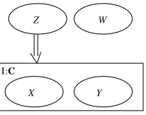
When specifying the relations among the variables, it may be difficult for the domain expert to indicate the presence or absence of edges between specific nodes in the model. If, for example, two variables X and Y in an instantiation I are strongly correlated, the domain expert may be uncertain whether another node Z in the encapsulating context of I should be the parent of X or Y (even though he believes that Z should influence at least one of them). In the OOBN framework, this prior infor-mation can be encoded by specifying the interface between the instantiation I and its encapsulating context. For instance, the domain expert can indicate which instantiations are allowed (and more importantly, denied) to reference a particular node (see Figure 8). Specifically, the domain expert could be asked questions like “Do you think it is possible that a variable Z directly influences any of the variables in instantiation I?”
Z
X Y
W
I:C
Figure 8: The figure depicts a possible way to describe knowledge about the structure of the do-main. It shows an instantiation I and some of its encapsulating context (note that this is not strictly speaking an OOBN).
have to encode that the probability for a link between Z and X depends on the existence of a link between Z and Y (the prior only penalizes a link missing between Z and X if there is no link from Z to Y ). This violates structural modularity, which says that the prior should factorize into a product of terms, where each term only depends on one family in the graph, see Section 3.2. On the other hand, if a candidate model is designed so that another node, say W , is referenced from I, it will be given a lower a priori belief (becauseω+XW =ωY W+ =ζ). Note that the OOBN framework is not required to model this vague prior information; it is merely a straight forward usage of Equation 8. However, to elicit such information it turns out to be useful to have grouped the nodes into what corresponds to instantiations, and then focus on the interfaces of these (working in the framework of OOBNs).
To verify the ease of determining the interfaces a priori we conducted an experiment amongst our co-workers: The task was to identify the interfaces of the instantiations in the object oriented version of the insurance domain, see Section 2.2. The test-persons were familiar with the OOBN framework, but they had not seen the insurance network before. Initially they were given the object oriented version of the insurance network, where each node was allocated to one of the instantia-tions (with all edges removed). The task was then to identify the interface of all instantiainstantia-tions in the domain, simply by indicating which nodes inside an instantiation Iicould (possibly) be referenced
from an instantiation Ij. The test-persons had no other information about the domain, except for
what they were able to deduce from the names of the nodes. They where guided through the knowl-edge acquisition by questions of the type “Is it possible that a person’s Age can directly influence any of the nodes in the instantiation of the Driver-class (RiskAversion, SeniorTrain, DrivingSkill, DrivQuality or DrivHist)?” The result of the experiment was that out of the 702 edges that can be included in the model, only 253 were marked possible. All the 52 edges actually in the model were considered legal. The elicitation of this information took about 10 minutes; this result at least suggests that the approach is promising.
5. Learning in OOBNs
In this section we describe a method for learning in object oriented domains, casted as the problem of finding the maximum a posteriori OOBN structure given a database
D
.The basic idea of the object oriented learning method resembles that of Langseth and Bangsø (2001) who exploit the OO assumption when learning the parameters in an OOBN. Specifically, based on this assumption, Langseth and Bangsø (2001) propose to learn at the class level of the OOBN instead of in the underlying BN; cases from the instantiations of a class are considered (virtual) cases of that class.9 Langseth and Bangsø (2001) give both theoretical as well as empirical evidence that this learning method is superior to conventional parameter learning in object oriented domains.
5.1 Structural OO Learning
The goal of our learning algorithm is to find a good estimate of the unknown underlying statistical distribution function. That is, we focus on the task of density estimation (Silverman, 1986). Note that if focus had been on, for example, causal discovery (Heckerman, 1995a), classification
man et al., 1997a), or generating a model that was able to predict well according to a predefined query distribution (Greiner et al., 1997), the learning method would have been slightly different (the general approach, however, would still apply).
The proposed method is tightly connected to the SEM-algorithm, described in Section 3.3. The main differences concern structure search and the calculation of the expected score of a network structure. When doing structure search we restrict the space of candidate structures by employing the search operations in the class specifications instead of in the underlying BN. This has the ad-vantages that i) the current best model is always guaranteed to be an OOBN, and ii) the learning procedure will in general require fewer steps than conventional learning because the search space is smaller.
The difference in the calculation of the expected score of an OOBN structure compared to a BN structure is a consequence of the OO assumption: Since we assume all instantiations of a given class to be identical, we treat cases from the instantiations of a given class as (virtual) cases of that class. Note that this approach can be seen as a generalization of the learning method for DBNs, described in Section 3.4, where all cases from the time-slices for t>0 are used for calculating the sufficient statistics for the transition network. Before giving a formal definition of the expected score of an OOBN structure we introduce the following notation (for now we shall assume that all input sets are empty): Let BCm be an OOBN for class Cm, and let{i : Xi∈C`}be the set of nodes defined in
class C`. Let
I
define the set of instantiations, let T(I)be the class of instantiation I∈I
, and let{I : T(I) =C`}be the set of instantiations of class C`(recall that we use I.X to denote node X in instantiation I).
The sufficient statistics Ni jkC`for a class C`, given a complete database, is then given by
Ni jkC`=
∑
I:T(I)=C`N
∑
t=1
γ(I.Xi=k,I.Πi=j : Dt). (9)
Based on the sufficient statistics for a class we can, under assumptions similar to those of Cooper and Herskovits (1991), derive the score for a node Xiin class C`as
O-score(Xi,Πi,NCi··`(
D
),C`) = qi∏
j=1
Γ(Ni j0)
Γ(Ni jC`+Ni j0)
ri
∏
k=1
Γ(Ni jkC`+Ni jk0 )
Γ(Ni jk0 ) , (10)
where NCi··`(
D
)specifies the collection Ni jkC`according toD
, and Ni jC`=∑rik=1N
C`
i jk.
Finally, we can define the BDe score for an OOBN BSas
P(
D
,BS|ξ)∝∏
C`∈
C
∏
i:Xi∈C`
ρ(Xi,Πi,C`)·O-score(Xi,Πi,NCi··`(
D
),C`), (11)where
C
is the set of all classes, andρ(Xi,Πi,C`)is a function of the prior specification of C`, suchthat
P(BS|ξ)∝
∏
C`∈
C
∏
i:Xi∈C`
ρ(Xi,Πi,C`).
In the situation with missing data we apply a modified version of the SEM algorithm. Recall that the SEM algorithm requires the calculation of
where o and h denote the observed and unobserved entries in
D
, respectively, and BnSis the current best model. In accordance with Equation 6 and Equation 11 we have (again we assume that the prior distribution is normalized)Eh[log P(o,h,BS)|BnS,o] =
∑
C`∈
C
∑
i:Xi∈C`
Eh[log Fi,C`(NCi··`(h,o),BS)|BnS,o] (12)
where
Fi,C`(NCi··`(h,o),BS) =ρ(Xi,Πi,C`)·O-score(Xi,Πi,NiC··`(h,o),C`).
Now, analogously to the SEM algorithm we advocate the approximation proposed in Equation 7 hence, for an OOBN we approximate
Eh[log Fi,C`(NiC··`(h,o),BS)|BSn,o]≈log Fi,C`(Eh[NCi··`(h,o)|B n
S,o],BS).
Finally, the expected countsEh[NCi··`(h,o)|BnS,o]for node Xiin class C`is given by
∀j,k :Eh[Ni jkC`(h,o)|BnS,o] =
∑
I:T(I)=C`N
∑
t=1
P(I.Xi=k,I.Πi= j|Dt,BnS).
Now, both Q(BS: BnS) and the posterior P(
D
,BS|ξ)factorize over the variables (and thereforealso over the classes). Hence, in order to compare two candidate structures which only differ w.r.t. the edge Xi→Xj we only need to re-calculate the score (Equation 10) andρ(Xj,Πj,C`)for node
Xj in the class C` where Xj is defined. Note that this property also supports the proposed search
procedure which is employed at the class level.
Unfortunately, this type of locality to a class is violated when the input sets are non-empty (this is for instance the case with the two instantiations of the class Milk Cow that are embedded in the
Stock class). The problem occurs when new input nodes are added to a class interface, since the
search for a “good” set of parents is not necessarily local to a class when the interface is not given. Recall that the actual nodes included through the interface of an instantiation is not defined in the class specification, but locally in each instantiation. This may result in a serious computational overhead when determining the interface since we require that the OO assumption is satisfied. As an example, assume that the node X in instantiation Ii is assigned an input node Y0 as parent, and
assume that Y0 references the node Y . Then, due to the OO assumption, the algorithm should find a node Z that has the same influence on Ij.X as Y has on Ii.X , for all instantiations Ij where
T(Ij) =T(Ii). The search for Z must cover all nodes in the encapsulating context of Ij. Note that
Z may be non-existent in which case the default potential for the input node should be used. The complexity of finding the best candidate interface for all instantiations is exponential in the number of instantiations, and we risk using a non-negligible amount of time to evaluate network structures with low score. For example if Y0 (or more precisely the node Y referenced by Y0) is actually not needed as a parent for Ii.X .
Algorithm 3 (OO–SEM)
a) Let B0Sbe the prior OOBN model. b) Loop for n=0,1,...until convergence
1) Compute the posterior P(ΘBnS|BnS,o), see Langseth and Bangsø (2001) and Green (1990).
2) Set BnS,0←BnS. 3) For i=0,1,...
i) Let BSbe the model which is obtained from BnS,iby employing either none or exactly
one of the operations add-edgeandremove-edge, for each instantiation I; each edge involved must have a node in both I and in the encapsulating context of I (directed into I). The OO assumption is disregarded.10
ii) For each node X, which is a child of an input node Y0 (found in step (i)) in instan-tiation Ij, determine if Ik.X has an input node as parent with the same state space
as Y0, for all k6= j where T(Ik) =T(Ij). If this is the case, use the BDe score to
determine if they should be assigned the same CPT (due to the OO assumption); otherwise introduce default potentials to ensure that they have the same CPTs.11 Let B0Sbe the resulting network.
iii) For each class C`in B0Semploy the operationsadd-edgeorremove-edgew.r.t. the nodes in the class (excluding the input set) based on the candidate interface found in step (ii). Note that edges from instantiations encapsulated in C`into nodes defined in C`are also considered in this step.12 Let B00Sbe the resulting OOBN.
iv) Set BnS,i+1←B00S.
4) Choose BnS+1←BnS,ithat maximizes Q(BnS,i: BnS)(Equation 12). 5) If Q(BnS: BnS) =Q(BnS+1: BnS)then
Return BnS.
Note that in Step (ii) it may seem counterintuitive to compare CPTs using the BDe score, however, observe that this step is actually used to restrict the parameter space and the BDe score is therefore appropriate, cf. the discussion in Section 3. Moreover, it should be noticed that we use strong type-checking in Step (ii), which ensures that the algorithm generates a legal OOBN as defined by Bangsø and Wuillemin (2000b). If we should learn an OOBN consistent with the definition of for example Koller and Pfeffer (1997), then stronger restrictions on the input sets would apply.
In case of a complete database, the outer loop is simply evaluated once; evaluating the network structures using Q(BS: BnS)is identical to using the BDe score for OOBNs in this case.
Theorem 1 Let
D
be a complete database of size N generated by an OOBN model with structure B∗S. If N→∞, then the structure BSreturned by Algorithm 3 is likelihood equivalent to B∗S.10. The number of operations is bounded by the product of the number of nodes in I and the number of nodes in the encapsulating context, but only the terms local to the involved families need to be re-calculated.
11. The CPTs are estimated by settingbθC` i jk=
NC`
i jk+Ni jk0
/NC` i j +Ni j0
, where NC`
i jkis the expected sufficient statistics
calculated according to Equation 9. Note that introducing default potentials have no effect on the underlying BN (they can just be marginalized out).
12. An example of this situation is illustrated in Figure 2.2, where an instantiation of Driver is encapsulated in the class
Proof Notice that the space of OOBN structures is finite, and that each OOBN structure can be
visited by the inner loop of Algorithm 3. Note also that the greedy approach in step (ii) is asymp-totically correct as the associated search space is uni-modal (as N→∞) and the operations are transitive. From these observations the proof is straightforward as the BDe score is asymptotically correct, see Heckerman (1995b) and Geiger et al. (1996).
Notice that the theorem above only holds when the database is complete. When the database is incomplete we have the following corollary.
Corollary 2 Let B0S,B1S,...be the sequence of structures investigated by Algorithm 3, and let
D
be a database. Then limn→∞P(o,BSn)exists, and it is a local maximum of P(o,BS)when regarded as afunction of BS.
Proof Follows immediately from Friedman (1998, Theorem 3.1 and Theorem 3.2) by observing that a) the space of OOBN structures is finite and the variables in the domain have discrete state spaces, and b) in Steps (i−iii) we are always sure to increase the expected score of the candidate model.
Observe that in order to complete the operational specification of Algorithm 3, we need a search algorithm, for instance simulated annealing, for investigating the candidate structures (Step (i) and Step (iii) constitute the choice points). Note also that in order to maximize the score in Step (ii) we would in principle need to investigate the set of all subsets of instantiations and nodes (which have an input node as parent). To avoid this computational problem we instead consider the instantiations and nodes pairwise (randomly chosen). This still ensures that the expected score increases in each iteration hence, the algorithm will converge even though we apply hill-climbing in Step (ii), see also Corollary 2.
Finally it should be emphasized that the main computational problem of Algorithm 3 is in establishing the interfaces of the instantiations hence, we propose to elicit prior information based on specific enquiries about the interfaces. For instance, the domain expert can be asked to specify the nodes each instantiation is allowed to reference; as argued in Section 4.2 this is easily elicitated in an object oriented domain. Prior information of the form “Daisy is to COW1 as Mathilda is to COW3”, related to the type-construct of Koller and Pfeffer (1997), can be exploited.
5.2 Type Uncertainty
So far we have assumed that the domain expert is able to unambiguously classify each instantiation to a specific class. Unfortunately, however, this may not be realistic in real-world applications. Not being able to classify an instantiation is an example of what is called type uncertainty by Pfeffer (2000); the expert is uncertain about the type (or class in our terminology) of an instantiation. However, even though we may be unable to determine whether, for instance, COW1 is a Milk cow or a Meat cow, see Section 2, we would still like to employ the learning algorithm using all available data.
When subject to type uncertainty the main problem is as follows. Consider the situation where we have two instantiations Ii and Ij whose classes are uncertain. Assume that both Iiand Ij are a
priori classified as being instantiations of Ck, and assume that the data from Ii and Ijare somewhat
is updated and the probability of Ij being an instantiation of Ck may therefore change. Thus, the
probability of Ij belonging to Ckis dependent on the classification of Ii. An immediate approach to
overcome this problem is brute force, where we consider all possible combinations of allocating the uncertain instantiations to the classes. However, this method is computationally very hard, and is not suited for practical purposes if the number of combinations of instantiations and classes is large. The complexity is O
|
C
||I
|.In what follows we propose an alternative algorithm for handling type uncertainty. We shall assume that the domain expert encodes his prior beliefs about the classification of the instan-tiations
I
as a distribution over the classesC
(this also allows us to restrict our search in the class tree to specific subtrees, if the domain expert encodes his prior belief in that way). Recall that the main problem with type uncertainty is that learning can only be performed locally in a class specification if all instantiations are allocated to a class (with certainty). This observation forms the basis for the following algorithm, which iteratively classifies the instantiations based on the MAP distribution over the classifications of the instantiations. Note that since the learned model is dependent on the classification of the uncertain instantiations, the algorithm maximizes the joint probability P(D
,BS(T
),T
), whereT
=T(I
); we use the notation BS(T
) to indicatethat the learned model is a function of the classifications. This probability can be computed as P(
D
,BS(T
),T
) =P(D
|BS(T
),T
)P(BS(T
)|T
)P(T
) where BS(T
) is a model consistent withthe classification
T
. In the following we will letT
b denote the current estimate of the classificationT(
I
). Furthermore, we useT
bI←C` to denote that the estimate of T(I) is set to C`, and we use bT
−Ito denote the estimate of T(I
\ {I}).Algorithm 4 (Type Uncertainty)
a) Initialization: Find the classification with maximum probability according to the prior
dis-tribution over the classifications P(T(
I
)), and classify the instantiations accordingly. LetT
b0be this initial classification.
b) Loop for n=0,1,...until convergence
1)
T
b0←T
bn.2) For each uncertain instantiation I:
i) For each classification C of I s.t. P(T(I) =C)>0:
A) Classify I as an instantiation of class C:
T
b0I←C.B) Learn the OOBN B0S(
T
b0)for the current classification of all instantiations(Al-gorithm 3).13Calculate the joint probability of the data, the model B0S(
T
b0)and bT
0:f(C)←P
D
,B0S(T
b0),T
b0. ii) Classify I to the class maximizing the joint probabilityP(
D
,B0S(T
b0),T
b0)by keeping the classifications T(I
\ {I})fixed: bT
0I←arg maxC:P(T(I)=C)>0f(C).3) Let
T
bn+1←T
b0and let BSn+1be the model found according to the classificationT
bn+1. 4) If P
D
,BnS+1(T
bn+1),T
bn+1=PD
,BnS(T
bn),T
bnthenReturn BnS(
T
bn).The algorithm attempts to maximize the joint probability P(
D
,BS(T
),T
)by iterativelymaxi-mizing 1) P(
D
,BS(T
b n),
T
bn)over the models BSwith the current classificationT
b n(Step B), and 2) P(
D
,BnS(T
b−nI,T(I)),(T
bn−I,T(I)))over T(I)given the classificationT
bn−I(Step ii). This also implies that the algorithm converges to a (local) maximum.6. Empirical Study
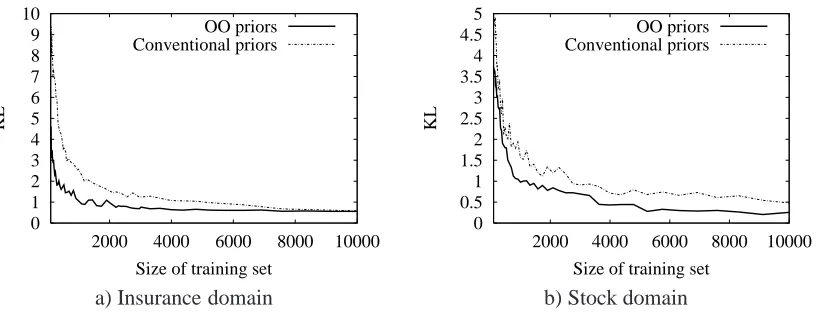
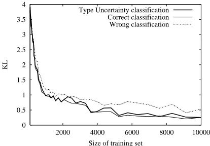
In this section we describe a set of empirical tests that have been conducted to verify the proposed learning method. First, Algorithm 3 was employed to learn the OOBN model of the insurance domain. This was done to identify the effect of prior information that is not easily exploited when the domain is not regarded as object oriented. Secondly, Algorithm 3 was employed on the stock domain to consider the effect of the OO assumption, and Algorithm 4 was used to verify the method for type uncertainty calculations. Finally, Algorithm 3 was tested w.r.t. predictive accuracy in the insurance domain.
6.1 Setup of the Empirical Study
The goal of the empirical study was to evaluate whether or not the proposed learning methods generate good estimates of the unknown statistical distribution. Let f(x|Θ)be the unknown gold standard distribution; x is a configuration of the domain andΘare the parameters. ˆfN(x|ΦˆN) (or
simply ˆfN) will be used to denote the approximation of f(x|Θ)based on N cases from the database.
Since an estimated model may have other edges than the gold standard model, the learned CPTs of ˆΦN may have other domains than the CPTs ofΘ. Hence a global measure for the difference
between the gold standard model and the estimated model is required. In the tests performed, we have measured this difference by using the Kullback-Leibler (KL) divergence (Kullback and Leibler, 1951) between the gold standard model and the estimated model. The KL divergence is defined as
D f||fˆN
=
∑
x
f(x|Θ)log
f(x|Θ) ˆfN(x|ΦˆN)
.
There are many arguments for using this particular measurement for calculating the quality of the approximation (see Cover and Thomas, 1991). One of them is the fact that the KL divergence bound the maximum error in the assessed probability for a particular event A, (Whittaker, 1990, Proposition 4.3.7):
sup
A
x
∑
∈Af(x|Θ)−x∑
∈AfˆN(x|ΦˆN)≤
r 1
2·D f||fˆN
.
Similar result for the maximal error of the estimated conditional distribution is derived by van Engelen (1997). These results have made the KL divergence the “distance measure”14 of choice 14. The KL divergence is not a distance measure in the mathematical sense, as D(f||g) =D(g||f)does not hold in