One-Class SVMs for Document Classification
Larry M. Manevitz [email protected]
Malik Yousef [email protected]
Department of Computer Science University of Haifa
Haifa 31905 Israel
Editors:Nello Cristianini, John Shawe-Taylor and Bob Williamson
Abstract
We implemented versions of the SVM appropriate for one-class classification in the context of information retrieval. The experiments were conducted on the standardReuters
data set.
For the SVM implementation we used both a version of Sch¨olkopf et al. and a somewhat different version of one-class SVM based on identifying “outlier” data as representative of the second-class. We report on experiments with different kernels for both of these imple-mentations and with different representations of the data, including binary vectors, tf-idf representation and a modification called “Hadamard” representation. Then we compared it with one-class versions of the algorithms prototype (Rocchio), nearest neighbor, naive Bayes, and finally a natural one-class neural network classification method based on “bot-tleneck” compression generated filters.
The SVM approach as represented by Sch¨olkopf was superior to all the methods except the neural network one, where it was, although occasionally worse, essentially comparable. However, the SVM methods turned out to be quite sensitive to the choice of representation and kernel in ways which are not well understood; therefore, for the time being leaving the neural network approach as the most robust.
Keywords: Support Vector Machine, SVM, Neural Network, Compression Neural Net-work, Text Retrieval, Positive Information
1. Introduction
Recently, mechanisms related to the Support Vector Machine (SVM) paradigm have pro-duced the dramatically best results for information retrieval, e.g. in experiments as mea-sured over the standardReuters dataset (Dumais et al., 1998).
Since Sch¨olkopf et al. (1999) recently extended the SVM methodology to handle training using only positive information (what they call “one-class” classification), we decided to apply their method to documentation classification and compare it with other one-class methods, including a method we recently developed and studied based on a compression neural network as a filter.
There are many parameters in these methods, including the representation of the data, and the decisions involved in modifying basically two-class methods to one class ones. Our studies are fairly broad although not completely comprehensive; below we describe each of the choices we made.
In the end, it turns out that the suggestion of Sch¨olkopf is quite excellent, substan-tially better than all other methods except the neural network based one with which it is comparable. Moreover, it is somewhat simpler to implement than the neural network method.
However, it turns out to be surprisingly sensitive to specific choices of representation and kernel in ways which are not very transparent. For example, the method works best with binary representation as opposed to tf-idf or “Hadamard” representations which are known to be superior in other methods. In addition, the proper choice of a kernel is dependent on the number of features in the binary vector. Since the difference in performance is very dramatic based on these choices, this means that the method is not robust without a deeper understanding of these representation issues.
This means that, for the moment, we would prefer the neural network method for reasons of robustness.
2. Document Representations, Data Set and Measurements
2.1 Document Representations
We used the following different representations in these experiments:
1. binary representation
2. frequency representation
3. tf-idfrepresentation
4. Hadamard representation
These are defined as follows. List all the words (after “stemming”; i.e. removing suffixes and prefixes to avoid duplicate entries and removing basic “stop” words) in all the training documents sorted by thedocument-frequency (i.e. the number of documents it appears in). Choose the topmsuch words according to this “dictionary” frequency (called “keywords”). (See in the sequel for experiments with different values ofm.)
Forbinaryrepresentation of a specific document, choose themdimensional binary vector where the ith entry is 1 if theith keyword appears in the document and 0 if it does not.
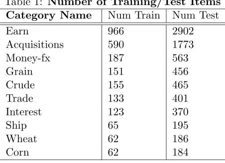
Table 1: Number of Training/Test Items Category Name Num Train Num Test
Earn 966 2902
Acquisitions 590 1773
Money-fx 187 563
Grain 151 456
Crude 155 465
Trade 133 401
Interest 123 370
Ship 65 195
Wheat 62 186
Corn 62 184
For thetf-idfrepresentation (“term frequency inverse document frequency”), choose the
m dimensional real valued vector, where theith entry is given by the formula
tf −idf(keyword) =f requency(keyword)·[log n
N(keyword) + 1].
where n is the total number of words in the dictionary and N is a function giving the total number of documents the keyword appears in.
The Hadamard product representation was discovered experimentally; it consists of the
mdimensional vector where the ith entry is the product of the frequency of theith keyword in the document and its frequency over all documents (in the training set). See Manevitz and Yousef (2001) for further discussion of this representation. In any case, it is clear that this transformation emphasizes differences between large and small feature entries.
2.2 Data Set and Measurements
To test the above ideas, we applied these filters to the standard Reuters dataset (Lewis, 1997), a preclassified collection of short articles. This is one of the standard test-beds used to test information retrieval algorithms (Dumais et al., 1998).
For each choice of category, we used 25% of the positive data from the training set to train; and then tested the filters on the remaining 75% of the data set. Table 1 shows the ten most frequent categories along with the number of training and test examples in each. We treated each of the 10 categories as a binary classification task and evaluated the classifiers for each category separately.
For reporting the results, we used the F1 measure, the recall and the precision values.
For text categorization, the effectiveness measure of recall and precision are defined as follows:
recall= Number of items of category identified
Number of category members in test set
precision= Number of items of category identified
Van Rijsbergen (1979) defined the F1-measure as a combination of recall (R) and
Pre-cision (P) with an equal weight in the following form: F1(R,P)= R2RP+P (This implies that
F1, like R and P, is bounded by 1 and the best results under this measure are the higher
values.)
3. SVM for One Class Classification: Separating Data from Origin
The SVM algorithm as it is usually construed is essentially a two-class algorithm (i.e. one needs negative as well as positive examples). Below we present two modifications, one due to Sch¨olkopf and one we proposed, to allow its use for only positive data. Both mechanisms identify “outliers” amongst the positive examples and use them as negative examples. Below we refer to the Sch¨olkopf method as “one-class” and to the other as “outlier”.
We investigated both algorithms under a variety of choices of parameters. Our exper-iments were more extensive for the one-class SVM which seems to be the superior of the two.
3.1 Sch¨olkopf Methodology
Sch¨olkopf et al. (1999) suggested a method of adapting the SVM methodology to the one-class one-classification problem. Essentially, after transforming the feature via a kernel, they treat the origin as the only member of the second class. Then using “relaxation parameters” they separate the image of the one class from the origin. Then the standard two-class SVM techniques are employed.
They framed the problem in the following way:
Suppose that a dataset has a probability distribution P in the feature space. Find a “simple” subset S of the feature space such that the probability that a test point fromP
lies outside S is bounded by some a priori specified value.
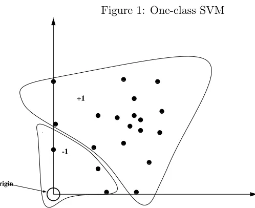
Supposing that there is a dataset drawn from an underlying probability distribution P, one needs to estimate a “simple” subsetS of the input space such that the probability that a test point from P lies outside of S is bounded by some a prior specified v∈(0,1) . The solution for this problem is obtained by estimating a functionf which is positive on S and negative on the complement S. In other words, Sch¨olkopf et al., developed an algorithm which returns a function f that takes the value +1 in a “small” region capturing most of the data vectors, and -1 elsewhere.
The algorithm can be summarized as mapping the data into a feature space H using an appropriate kernel function, and then trying to separate the mapped vectors from the origin with maximum margin (see Figure 1).
f(x) =
+1 if x∈S
−1 if x∈S
In our context, let x1, x2, . . . , xl be training examples belonging to one class X, where
Figure 1: One-class SVM
One-Class SVM Classifier. The origin is the only original member of the second class. 00 00 00 11 11 11 00 00 00 11 11 11 00 00 00 11 11 11 00 00 11 11 00 00 11 11 00 00 00 11 11 11 0 0 0 1 1 1 0 0 1 1 00 00 11 11 0 0 1 1 0 0 0 1 1 1 00 00 11 11 00 00 00 11 11 11 0 0 1 1 00 00 00 11 11 11 0 0 0 1 1 1 00 00 11 11 00 00 00 11 11 11 00 00 00 11 11 11 0 0 1 1 Origin -1 +1 min1
2w
2+ 1
vl
l
i=1
ξi−ρ
subject to
(w·Φ(xi))≥ρ−ξi i= 1,2, ..., l ξi≥0
If wand ρ solve this problem, then the decision function
f(x) =sign((w·Φ(x))−ρ)
will be positive for most examplesxi contained in the training set.
In our research we used the LIBSVM (version 2.0). This is an integrated tool for support vector classification and regression which can handle one-class SVM using the Sholkopf etc algorithms. The LIBSVM 2.0 is available at http://www.csie.ntu.edu.tw/˜cjlin/libsvm. We used the standard parameters of the algorithm.
For this “one-class SVM”, one has to choose the original frequency representation, (e.g. the number of features), the appropriate kernel, and for each kernel the appropriate param-eters. We allowed, linear, sigmoid, polynomial and radial basis kernels; each chosen with the standard parameters. For the original feature representation, we used binary, tf-idf and Hadamard representations. For the number of features we tried 10, 20, 40, 60 and 100 features for the one-class SVM.
3.2 Outlier Methodology
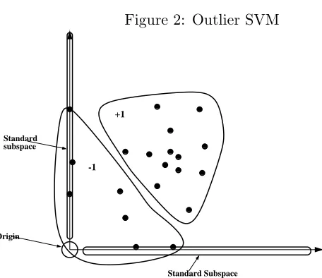
Figure 2: Outlier SVM
of the second class. The diagram is conceptual only.
Outlier SVM Classifier. The origin and small subspaces are the original members
0 0 0 1 1 1 0 0 1 1 0 0 0 1 1 1 0 0 1 1 0 0 1 1 0 0 1 1 0 0 0 1 1 1 00 00 11 11 00 00 11 11 00 00 11 11 00 00 00 11 11 11 00 00 11 11 00 00 00 11 11 11 00 00 11 11 0 0 0 1 1 1 0 0 0 1 1 1 00 00 11 11 0 0 1 1 00 00 11 11 Standard subspace +1 -1 Origin Standard Subspace 0 0 1 1
If a vector has few non-zero entries, then this indicates that this document shares very few items with the chosen feature subset of the dictionary. So, intuitively, this item will not serve well as a representative of the class. In this way, it is reasonable to treat such a vector as an outlier. (Note that while the idea of choosing the outliers as data points close to the origin is a general one, the intuitive justification of this procedure is specific to this application.)
Geometrically, using the Hamming distance means that all vectors lying on standard sub-spaces of small dimension (i.e. axes, faces, etc.) are treated as outliers (see Figure 2).
Hence, we decided to identify these outliers by counting the features of an example with non-zero value; and if this is less than a threshold, then the feature is labeled as a negative example.
This raises the problem as to how to choose the appropriate values for the threshold. We investigated this in two ways: (1) by experimentally trying different global values of the threshold and (2) by determining individual thresholds for the different categories. One should note that, in principle, this determination of threshold can be done automatically, e.g. by comparing results on a test set. After having determined the threshold one then continues with the standard two-class SVM.
For this “outlier-SVM”, one also has to choose the original frequency representation, and how far from the origin a point can be (in our case, in Hamming distance) before being classified as an outlier.
For the outlier-SVM we tried 10 and 20 features for binary representations. Note that the features are individual category-specific, i.e. different features for each category. (We did sample runs with other representations (e.g. Hadamard, tf-idf) and larger numbers of features, but since the results were clearly poor, we did not complete the experiments.)
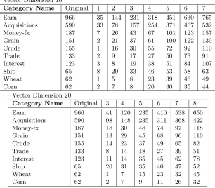
each category had its own such threshold. Table 6 lists the number of documents designated as outliers for each choice of Hamming distance.
We allowed, linear, sigmoid, polynomial and radial basis kernels; each chosen with the “standard” parameters for the two class SVM.
4. Other Methods
In recent research (Manevitz and Yousef, 2001) we proposed a one-class neural network classification scheme and compared it over the standard Reuters data set with variants appropriate to the positive example case of several algorithms, using various choices of parameters and various methods of representing the details. For extensive details, see Manevitz and Yousef (2001).
Here we will compare the two SVM one-class algorithms with the following ones from that study:
1. Prototype (Rocchio’s) algorithm
The Prototype algorithm is widely used in information retrieval (Pazzani and Billsus, 1997, Balabanovic and Shoham, 1995, Pazzani et al., 1996, Lang, 1995, and others) . This algorithm is used frequently because it is considered as a baseline algorithm and it is simple to implement. For more details see Joachims (1996).
The basic idea of the algorithm is to represent each document, e, as a vector in a vector space so that documents with similar content have similar vectors. The value
ei of the ith key-word is represented as thetf-idf weight.
The Prototype algorithm learns the class model by combining document vectors into a prototype vector . This vector is generated by adding the document vectors of all documents in the class. Classification is done by judging the angular distance from the prototype vector. In our experiments, we used the F1 measure to optimize the
threshold.
2. Nearest Neighbor
This is a modification of the standard Nearest Neighbor algorithm (Yang and Liu, 1999) appropriate for one-class learning. This algorithm was original presented in detail by Datta (1997); and the method of optimizing the parameters is explained by Manevitz and Yousef (2001).
3. Naive Bayes
Traditional Naive Bayes calculates the probability of being in a class given an example, which has specific values for the different attributes. One calculates this by assuming the different attributes are independent, applying Bayes’ theorem and using the a priori probability of the different classes.
P. Datta (1997) showed how to modify the algorithm for positive data only and we follow his presentation.
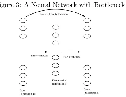
Figure 3: A Neural Network with Bottleneck
Trained Identity Function
Input
Compression (dimension k)
Output (dimension m) (dimension m)
fullly connected fully connected
estimated independently using the formula: p(w|E) = nw+1
n+m wherenw is the number
of times wordwoccurs inE,nis the total number of words inE, andmis the number of keywords.
The threshold is calculated as a fraction (optimized using the F1 measure) of the
minimum over all examples inE of the valuep(d|E)
4. Compression Neural Network
The algorithm is based on a feed-forward three layer neural network with a “bot-tleneck”. That is, under the assumption that the documents are represented in an
m-dimensional space; we choose a three level network withm inputs, m outputs and
kneurons on the hidden level, wherek < m. Then the network is trained, under stan-dard back-propagation, to learn the identity function on the sample examples (see Figure 3). This design was first used by G.W. Cottrell and Zipser (1988) to produce a compression algorithm. See also Japkowicz et al. (1995) for another use as a novelty detector.
The idea is that while the bottleneck prevents learning the full identity function on
m-space; the identity on the small set of examples is in fact learnable. Then the set of vectors for which the network acts as the identity function is a sort of sub-space which is similar to the trained set. This avoids the “saturation” problem of learning from only positive examples. Thus the filter is defined by applying the network to a given vector; if the result is the identity, then the vector is “interesting”.
By running the same experiments using the two SVM-one class algorithms, we are in a position to make a comparative study.
The reader is referred to Manevitz and Yousef (2001) for detailed descriptions of each of the above algorithms and the various choices of parameters investigated.
5. Results
We present our results in a series of tables listing the F1, recall and precision values over
5.1 One-class SVM (Sch¨olkopf algorithm) Results
The results for this algorithm were very sensitive to the parameters. However, under proper choices it can give the best results.
In particular:
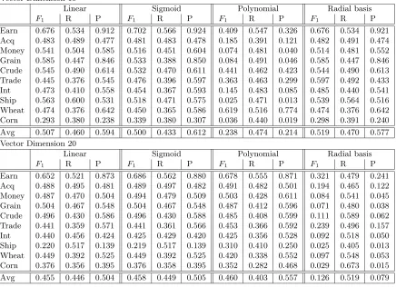
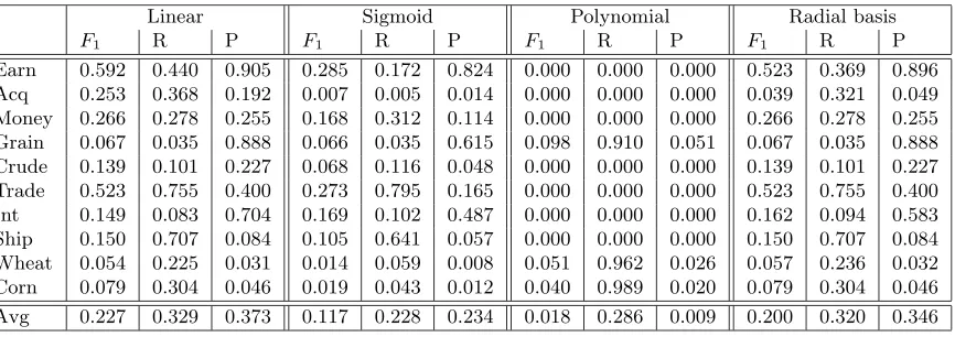
• This algorithm worked much better with the binary representation; in fact the results under all kernels were extremely poor under the other three representations we tested (frequency, tf-idf, and Hadamard). Table 5 presents the Hadamard results with 20 features; results with tf-idf and frequency were equally poor.
• 10 features were best in general, but this depended on the choice of kernel. For polynomial kernel the 20 features were dramatically better. On the other hand, for radial basis kernel 10 features were dramatically better than 20 features (see Table 3).
• Increasing the number of features further caused large decreases in performance (see Table 4).
Aside: Note that the features are category-specific in our approach; unlike other stud-ies such as performed by Joachims (1998), for example. This makes direct dimension comparison difficult. Roughly, the total number of features over all categories in our experiments is about 100 (for twenty features per category).
• We investigated the effect of removing the near-Hamming distance examples from the data set before running this algorithm. We did this for vectors with 10 features. Since the results are worse in all cases in comparison with the original algorithm, we do not reproduce the data tables here.
In summary, the best choice of parameters for this algorithm were 10 features, binary representation with radial basis kernel. However, the sensitivity to changes in any of these parameters makes it difficult to generalize to other applications. The linear kernel, however, while giving somewhat worse results did not seem to be as sensitive.
5.2 Outlier-SVM Results
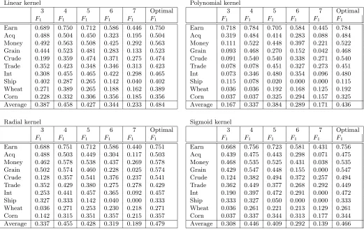
The results were generally somewhat worse than the one-class SVM results reported above, especially when looked over the array of categories. Occasionally, (e.g. for polynomial kernel with 10 features) this method was superior. Compare Table 3 with Table 2.
For larger categories, outlier-SVM obtained somewhat better results. Using macro av-eraging (i.e. taking into account the differing number of items in each category), this algorithm reports somewhat better results than the one-class SVM (see Table 8).
• We only tested this algorithm for binary representation.
• 10 features were preferable to 20 features. Compare Table 7 and the subtables in Table 2.
Table 2: F1 Values for the Outlier-SVM with different kernels. All with binary
representa-tion and vector dimension 10. The number in the first row indicates the number of non-zero feature entries which is required to consider an object an outlier.
Linear kernel
3 4 5 6 7 Optimal
F1 F1 F1 F1 F1 F1
Earn 0.689 0.750 0.712 0.586 0.446 0.750
Acq 0.488 0.504 0.450 0.323 0.195 0.504
Money 0.492 0.563 0.508 0.425 0.292 0.563
Grain 0.444 0.523 0.481 0.283 0.133 0.523
Crude 0.199 0.359 0.474 0.371 0.275 0.474
Trade 0.352 0.423 0.348 0.346 0.313 0.423
Int 0.308 0.455 0.465 0.422 0.298 0.465
Ship 0.402 0.287 0.265 0.142 0.040 0.402
Wheat 0.271 0.389 0.265 0.188 0.162 0.389
Corn 0.228 0.332 0.306 0.356 0.185 0.356
Average 0.387 0.458 0.427 0.344 0.233 0.484
Polynomial kernel
3 4 5 6 7 Optimal
F1 F1 F1 F1 F1 F1
Earn 0.718 0.784 0.705 0.584 0.445 0.784
Acq 0.319 0.484 0.414 0.283 0.088 0.484
Money 0.111 0.522 0.448 0.397 0.221 0.522
Grain 0.093 0.468 0.270 0.152 0.042 0.468
Crude 0.091 0.540 0.540 0.338 0.271 0.540
Trade 0.078 0.078 0.451 0.327 0.273 0.451
Int 0.073 0.346 0.480 0.354 0.096 0.480
Ship 0.115 0.078 0.020 0.000 0.000 0.115
Wheat 0.036 0.036 0.192 0.168 0.125 0.192
Corn 0.037 0.037 0.325 0.294 0.157 0.325
Average 0.167 0.337 0.384 0.289 0.171 0.436
Radial kernel
3 4 5 6 7 Optimal
F1 F1 F1 F1 F1 F1
Earn 0.688 0.751 0.712 0.586 0.440 0.751
Acq 0.488 0.503 0.449 0.304 0.117 0.503
Money 0.462 0.578 0.538 0.437 0.269 0.578
Grain 0.502 0.574 0.460 0.228 0.025 0.574
Crude 0.128 0.357 0.541 0.376 0.237 0.541
Trade 0.352 0.429 0.380 0.275 0.278 0.429
Int 0.253 0.441 0.457 0.365 0.092 0.457
Ship 0.327 0.333 0.142 0.040 0.000 0.333
Wheat 0.036 0.271 0.253 0.230 0.218 0.271
Corn 0.142 0.315 0.351 0.357 0.215 0.357
Average 0.337 0.455 0.428 0.319 0.189 0.479
Sigmoid kernel
3 4 5 6 7 Optimal
F1 F1 F1 F1 F1 F1
Earn 0.668 0.756 0.723 0.581 0.431 0.756
Acq 0.439 0.475 0.443 0.298 0.071 0.475
Money 0.468 0.535 0.525 0.431 0.038 0.535
Grain 0.429 0.547 0.448 0.155 0.000 0.547
Crude 0.124 0.382 0.494 0.372 0.257 0.494
Trade 0.362 0.449 0.377 0.268 0.292 0.449
Int 0.190 0.397 0.472 0.291 0.000 0.472
Ship 0.333 0.327 0.050 0.000 0.000 0.333
Wheat 0.036 0.261 0.221 0.213 0.129 0.261
Corn 0.037 0.337 0.344 0.313 0.177 0.344
Table 3: One-class SVM using the binary representation.
Vector Dimension 10
Linear Sigmoid Polynomial Radial basis
F1 R P F1 R P F1 R P F1 R P
Earn 0.676 0.534 0.912 0.702 0.566 0.924 0.409 0.547 0.326 0.676 0.534 0.921
Acq 0.483 0.489 0.477 0.481 0.483 0.478 0.185 0.391 0.121 0.482 0.491 0.474
Money 0.541 0.504 0.585 0.516 0.451 0.604 0.074 0.481 0.040 0.514 0.481 0.552
Grain 0.585 0.447 0.846 0.533 0.388 0.850 0.084 0.491 0.046 0.585 0.447 0.846
Crude 0.545 0.490 0.614 0.532 0.470 0.611 0.441 0.462 0.423 0.544 0.490 0.613
Trade 0.445 0.376 0.545 0.476 0.396 0.597 0.363 0.463 0.299 0.597 0.492 0.433
Int 0.473 0.410 0.558 0.454 0.367 0.593 0.145 0.483 0.085 0.485 0.440 0.541
Ship 0.563 0.600 0.531 0.518 0.471 0.575 0.025 0.471 0.013 0.539 0.564 0.516
Wheat 0.474 0.376 0.642 0.450 0.365 0.586 0.619 0.516 0.774 0.474 0.376 0.642
Corn 0.293 0.380 0.238 0.339 0.380 0.307 0.036 0.440 0.019 0.298 0.391 0.240
Avg 0.507 0.460 0.594 0.500 0.433 0.612 0.238 0.474 0.214 0.519 0.470 0.577
Vector Dimension 20
Linear Sigmoid Polynomial Radial basis
F1 R P F1 R P F1 R P F1 R P
Earn 0.652 0.521 0.873 0.686 0.562 0.880 0.678 0.555 0.871 0.321 0.479 0.241
Acq 0.488 0.495 0.481 0.489 0.497 0.482 0.491 0.482 0.501 0.194 0.465 0.122
Money 0.487 0.470 0.504 0.494 0.479 0.509 0.503 0.428 0.611 0.084 0.541 0.045
Grain 0.504 0.467 0.548 0.504 0.467 0.548 0.487 0.412 0.596 0.071 0.480 0.038
Crude 0.496 0.430 0.586 0.496 0.430 0.588 0.485 0.408 0.599 0.111 0.589 0.062
Trade 0.441 0.359 0.571 0.441 0.361 0.566 0.453 0.366 0.592 0.239 0.496 0.157
Int 0.440 0.456 0.424 0.425 0.429 0.420 0.425 0.356 0.528 0.092 0.518 0.050
Ship 0.220 0.517 0.139 0.219 0.517 0.139 0.310 0.410 0.250 0.025 0.405 0.013
Wheat 0.449 0.392 0.525 0.449 0.392 0.525 0.420 0.338 0.552 0.097 0.548 0.053
Corn 0.376 0.356 0.395 0.376 0.358 0.395 0.352 0.282 0.468 0.029 0.673 0.015
Avg 0.455 0.446 0.504 0.458 0.449 0.505 0.460 0.403 0.557 0.126 0.519 0.079
Table 4: One-class SVM using the binary representation, with different vector dimensions. Some sample categories.
Linear Sigmoid Polynomial Radial basis
F1 R P F1 R P F1 R P F1 R P
dimension 40
Grain 0.479 0.453 0.707 0.425 0.331 0.594 0.059 0.524 0.031 0.478 0.453 0.506
Ship 0.135 0.482 0.078 0.203 0.205 0.202 0.027 0.589 0.014 0.135 0.482 0.078
Wheat 0.416 0.392 0.442 0.307 0.226 0.482 0.030 0.548 0.015 0.414 0.392 0.439
Corn 0.340 0.380 0.308 0.325 0.250 0.464 0.029 0.625 0.015 0.339 0.380 0.307
dimension 60
Grain 0.436 0.434 0.438 0.398 0.300 0.593 0.056 0.486 0.029 0.434 0.434 0.435
Ship 0.177 0.400 0.114 0.229 0.169 0.358 0.029 0.671 0.014 0.178 0.405 0.014
Wheat 0.383 0.381 0.385 0.254 0.182 0.419 0.028 0.591 0.014 0.388 0.387 0.389
Corn 0.326 0.347 0.307 0.272 0.195 0.450 0.027 0.592 0.013 0.324 0.347 0.303
dimension 100
Grain 0.412 0.425 0.400 0.259 0.157 0.727 0.031 0.232 0.017 0.412 0.425 0.400
Ship 0.164 0.446 0.100 0.150 0.092 0.400 0.028 0.625 0.014 0.164 0.446 0.100
Wheat 0.530 0.376 0.897 0.258 0.150 0.903 0.039 0.634 0.020 0.530 0.376 0.897
Table 5: One-class SVM using the Hadamard representation, with vector dimension 20 (m=20).
Linear Sigmoid Polynomial Radial basis
F1 R P F1 R P F1 R P F1 R P
Earn 0.592 0.440 0.905 0.285 0.172 0.824 0.000 0.000 0.000 0.523 0.369 0.896
Acq 0.253 0.368 0.192 0.007 0.005 0.014 0.000 0.000 0.000 0.039 0.321 0.049
Money 0.266 0.278 0.255 0.168 0.312 0.114 0.000 0.000 0.000 0.266 0.278 0.255
Grain 0.067 0.035 0.888 0.066 0.035 0.615 0.098 0.910 0.051 0.067 0.035 0.888
Crude 0.139 0.101 0.227 0.068 0.116 0.048 0.000 0.000 0.000 0.139 0.101 0.227
Trade 0.523 0.755 0.400 0.273 0.795 0.165 0.000 0.000 0.000 0.523 0.755 0.400
Int 0.149 0.083 0.704 0.169 0.102 0.487 0.000 0.000 0.000 0.162 0.094 0.583
Ship 0.150 0.707 0.084 0.105 0.641 0.057 0.000 0.000 0.000 0.150 0.707 0.084
Wheat 0.054 0.225 0.031 0.014 0.059 0.008 0.051 0.962 0.026 0.057 0.236 0.032
Corn 0.079 0.304 0.046 0.019 0.043 0.012 0.040 0.989 0.020 0.079 0.304 0.046
Avg 0.227 0.329 0.373 0.117 0.228 0.234 0.018 0.286 0.009 0.200 0.320 0.346
as outliers. This indicates that it would be useful to find a better criteria for the original specification of keywords. This is somewhat difficult because in our context only positive information is available.
In summary, the best parameters for this algorithm were binary representation, feature length 10, and linear kernel function (there was not much difference from the radial basis kernel).
6. Comparisons and Conclusions
In Table 8, we list the best F1 results from one-class SVM, outlier-SVM and the four other
algorithms from the work by Manevitz and Yousef (2001). The results from ten Reuters categories are presented. We also list, in this table, the “macro” averages which take into account the different number of items in each category.
Looking over this table, and focusing on the unweighted average, we see that the one-class SVM as proposed by Sch¨olkopf et al., gives the best overall performance. This is quite clear with respect to all the other algorithms except the compression NN algorithm which is comparable. Sch¨olkopf’s proposal has the usual advantages of SVM; in particular it is less computationally intensive than neural networks.
Under the “macro” averaging, the NN and outlier-SVM were somewhat superior. This means that while the one-class SVM was more robust with regards to smaller categories, the NN and outlier-SVM showed good results by emphasizing success in the larger categories.
Table 6: Cumulative number of negative examples (outliers) used from the training set to train the outlier-SVM classifier.
Vector Dimension 10
Category Name Original 1 2 3 4 5 6 7
Earn 966 35 144 231 318 451 630 765
Acquisitions 590 33 78 157 254 371 467 532
Money-fx 187 7 26 43 67 101 123 157
Grain 151 2 21 37 61 100 122 139
Crude 155 1 16 30 55 72 92 110
Trade 133 2 9 17 27 50 73 91
Interest 123 3 8 19 38 51 84 107
Ship 65 8 20 33 46 53 58 63
Wheat 62 1 5 8 23 39 46 49
Corn 62 2 7 8 20 30 35 44
Vector Dimension 20
Category Name Original 3 4 5 6 7 8
Earn 966 41 120 235 410 538 650
Acquisitions 590 98 148 235 311 368 422
Money-fx 187 18 30 48 74 97 118
Grain 151 13 29 45 68 96 110
Crude 155 14 23 37 49 65 82
Trade 133 8 14 18 27 39 51
Interest 123 11 14 35 45 62 78
Ship 65 20 31 35 40 47 52
Wheat 62 1 7 15 23 32 45
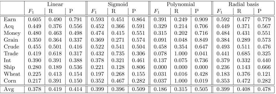
Table 7: Outlier-SVM using binary representation with different kernel functions, outliers with Hamming distance 7, vector dimension 20.
Linear Sigmoid Polynomial Radial basis
F1 R P F1 R P F1 R P F1 R P
Earn 0.605 0.490 0.791 0.593 0.451 0.864 0.391 0.249 0.909 0.592 0.477 0.779
Acq 0.449 0.376 0.556 0.452 0.366 0.591 0.329 0.214 0.706 0.449 0.371 0.567
Money 0.480 0.463 0.498 0.474 0.415 0.551 0.315 0.202 0.716 0.484 0.431 0.551
Grain 0.350 0.364 0.337 0.369 0.271 0.574 0.091 0.048 0.849 0.384 0.289 0.573
Crude 0.455 0.501 0.416 0.522 0.541 0.504 0.458 0.354 0.647 0.493 0.511 0.476
Trade 0.419 0.618 0.317 0.432 0.735 0.306 0.078 1.000 0.041 0.441 0.685 0.325
Int 0.390 0.391 0.388 0.378 0.321 0.461 0.137 0.075 0.736 0.379 0.332 0.440
Ship 0.280 0.189 0.536 0.221 0.128 0.806 0.000 0.000 0.000 0.236 0.143 0.666
Wheat 0.225 0.413 0.154 0.197 0.268 0.155 0.031 0.016 0.428 0.183 0.376 0.121
Corn 0.217 0.391 0.150 0.352 0.467 0.282 0.037 1.000 0.019 0.353 0.472 0.282
Avg 0.378 0.419 0.414 0.399 0.396 0.509 0.186 0.315 0.505 0.399 0.408 0.478
Table 8: Comparison of One-class SVM (binary representation), Outlier-SVM (binary rep-resentation), Neural Networks (Hadamard reprep-resentation), Naive Bayes, Nearest Neighbor (Hadamard representation), and Prototype Algorithms (tf-idf represen-tation). (Each method with the best representation tested.)
One-class Outlier- Neural Naive Nearest Prototype
SVM Radial SVM Networks Bayes Neighbor
Basis Linear
F1 F1 F1 F1 F1 F1
Earn 0.676 0.750 0.714 0.708 0.703 0.637
Acq 0.482 0.504 0.621 0.503 0.476 0.468
Money 0.514 0.563 0.642 0.493 0.468 0.484
Grain 0.585 0.523 0.473 0.382 0.333 0.402
Crude 0.544 0.474 0.534 0.457 0.392 0.398
Trade 0.597 0.423 0.569 0.483 0.441 0.557
Int 0.485 0.465 0.487 0.394 0.295 0.454
Ship 0.539 0.402 0.361 0.288 0.389 0.370
Wheat 0.474 0.389 0.404 0.288 0.566 0.262
Corn 0.298 0.356 0.324 0.254 0.168 0.230
Avg 0.519 0.484 0.513 0.425 0.423 0.426
Macro 0.572 0.587 0.615 0.547 0.530 0.516
Acknowledgments
References
M. Balabanovic and Y. Shoham. Learning information retrieval agents: Experiments with automated web browsing. In Working Notes of AAAI Spring Symposium Series on In-formation Gathering from Distributed, Heterogeneous Environments. AAAI-Press, 1995.
P. Datta. Characteristic Concept Representations. PhD thesis, University of California, Irvine, 1997.
S.T. Dumais, J. Platt, D. Heckerman, and M. Sahami. Inductive learning algorithms and representation for text categorization. In Proceedings of the seventh International Con-ference on Information and Knowledge Management (CIKM’98), pages 148–155, 1998.
P. Munro G.W. Cottrell and D. Zipser. Image compression by back propagation: an example of extensional programming. In N.E. Sharkey, editor, Advances in Cognitive Science, volume 3. Ablex, 1988.
N. Japkowicz, C. Myers, and M. Gluck. A novelty detection approach to classification. In
Proceeding of the Fourteenth International Conference On Artificial Intelligence, pages 518–523. Montreal, Canada, 1995.
T. Joachims. A probabilistic analysis of the Rocchio algorithm with TF-IDF for text cat-egorization. Technical Report CMU-CS-96-118, School of Computer Science, Carnegie Mellon University, Pittsburgh, 1996.
T. Joachims. Text categorization with support vector machines: Learning with many relevant features. In Proceeding 10 European Conference on Machine Learning (ECML), pages 137–142. Springer Verlag, 1998. URL
http://www-ai.cs.uni-dortmund.de/DOKIMENTE/Joachims 97a.sp.gz.
K. Lang. NewsWeeder:Learning to filter news. In Twelfth International Conference on Machine Learning, pages 331–339. Lake Tahoe, CA, 1995.
D. Lewis. Reuters-21578 text categorization test collection.
http://www.research.att.com/~lewis, 1997.
L. Manevitz and M. Yousef. Document classification via neural networks trained exclusively with positive examples. Technical report, Department of Computer Science, University of Haifa, Haifa, 2001.
M. Pazzani and D. Billsus. Learning and revising user profiles: The identification of inter-esting web sites. Machine Learning, 27:313–331, 1997.
M. Pazzani, J. Muramatsu, and D. Billsus. Syskill & Webert:Identifying interesting web sites. In AAAI Conference 1996, pages 54–61, 1996.
C.J. van Rijsbergen. Information Retrieval. Butterworths, London, second edition, 1979.
Yiming Yang and Xin Liu. A re-examination of text categorization methods. In Marti A. Hearst, Fredric Gey, and Richard Tong, editors, Proceedings of SIGIR-99, 22nd ACM International Conference on Research and Development in Informa-tion Retrieval, pages 42–49, Berkeley, US, 1999. ACM Press, New York, US. URL