Application of Generalized Integral Representation (GIRM) Method to Fluid Dynamic Motion of Gas or Particles in Cosmic Space Driven by Gravitational Force

(1)

Applied and Computational Mathematics

2015; 4(3-1): 15-39

Published online February 10, 2015 (http://www.sciencepublishinggroup.com/j/acm) doi: 10.11648/j.acm.s.2015040301.12

ISSN: 2328-5605 (Print); ISSN: 2328-5613 (Online)

Application of generalized integral representation (GIRM)

method to fluid dynamic motion of gas or particles in

cosmic space driven by gravitational force

Hiroshi Isshiki

1

, Toshio Takiya

2

, Hideyuki Niizato

2 1

IMA, Institute of Mathematical Analysis, Osaka, Japan 2

Hitachi Zosen Corporation, Osaka, Japan

Email address:

[email protected] (H. Isshiki), [email protected] (T. Takiya), [email protected] (H. Niizato)

To cite this article:

Hiroshi Isshiki, Toshio Takiya, Hideyuki Niizato. Application of Generalized Integral Representation (GIRM) Method to Fluid Dynamic Motion of Gas or Particles in Cosmic Space Driven by Gravitational Force. Applied and Computational Mathematics. Special Issue: Integral Representation Method and its Generalization. Vol. 4, No. 3-1, 2015, pp. 15-39. doi: 10.11648/j.acm.s.2015040301.12

Abstract:

Some aspect of the motion of gas or vast-number-of-particles distributed in cosmic space under action of the gravitational force may be treated as a fluid dynamic motion without pressure. Generalized Integral representation Method (GIRM) is applied to fluid dynamic motion of gas or particles to obtain the accurate numerical solutions. In the present theory, the relativistic effects are neglected. The numerical results by GIRM are compared with the solutions by Finite Difference Method (FDM). Spreading and merging of gas or particles and effects of initial velocity distribution are studied numerically. GIRM solutions give reasonable and accurate solutions.

Keywords:

Formation of Star, Gravitational Force, Gas, Particle, Fluid Dynamic Approximation

1. Introduction

In the process of the star formation in early cosmos, the vast number of particles were distributed in the cosmic space almost uniformly, and the stars were formed under the action of the gravitational force [1]. Some aspect of the motion of particles may be treated as a fluid dynamic motion without pressure [2,3]. The fluid dynamic approach may simplify the theory and numerical simulation. In the present theory, the relativistic effects are neglected, since it is not so important in the following studies. General integral representation method (GIRM) was applied to the numerical calculations below. Spreading and merging of gas or particles and effects of initial velocity distribution are studied numerically. The numerical results by GIRM are compared with the solutions by Finite Difference Method (FDM). GIRM solutions give reasonable and accurate solutions.

2. One-Dimensional Fluid Motion

without Pressure

Some aspect of motion of gas or vast number of particles distributed in space under the action of the gravitational force

may be treated as a fluid dynamic motion without pressure

[2,3]. If

x

and

t

refer to the coordinates and time, the

fluid motion is expressed as

0

= ∂ ∂ + ∂ ∂

x u t

ρ ρ

, (1)

2 2

x u x x u u t u

∂ ∂ + ∂

Π ∂ − = ∂ ∂ + ∂

∂ _ν _{, (2)}

ρ πG x2 4 2

= ∂

Π ∂

, (3)

where ρ, ν , u and Π is the mass density, kinematic

viscosity, velocity and gravitational potential (Appendix A).

G is the gravitational constant.

We introduce Gaussian type Generalized Fundamental Solution (GFM) G~(x,ξ) with scale γ [4,5]:

    

 

 ₋

−

= 2

2

2 ) ( exp 2

1 ) , ( ~

γ ξ γ

π

ξ x

x

(2)

16 Hiroshi Isshiki et al.: Application of Generalized Integral Representation (GIRM) Method to Fluid Dynamic Motion of Gas or Particles in Cosmic Space Driven by Gravitational Force

      ₋ − − − = ∂ ∂ 2 2 3 ₂ ) ( exp 2 ) , ( ~ γξ γ π ξ

ξ x x

x x G

, (4b)

2 2

2 3 2

2 2

2 5

( , ) 1 ( )

exp 2 2 ( ) ( ) exp 2 2

G x x

x x x ξ ξ γ π γ ξ ξ γ π γ   ∂ _{= −} ₋ −   ∂     − − + −    ɶ

. (4c)

First, we obtain an integral representation of the equation of continuity given by Eq. (1). For the purpose, we notice

( , ) ( , ) ( , ) ( , ) ( , )

( , )

( , ) ( , ) ( , )

x t u x t x t u x t G x G x

x x

G x x t u x t

x

ρ _ξ ρ ξ

ξ ρ ∂ ₌∂ ∂ ∂ ∂ − ∂ ɶ ɶ

ɶ . (5)

Multiplying G~(x,ξ) on the both sides of Eq. (1) and

integrating in region 0<x<L, we obtain

0

0 0

0

( , ) ( , ) ( , )

0 ( , )

( , ) ( , ) ( , ) ( , ) ( , ) ( , ) ( , ) ( , ) L L L L

x t x t u x t

G x dx

t x

x t x t u x t G x

G x dx dx

t x

G x x t u x t dx

x

ρ ρ _ξ

ρ _ξ ρ ξ

ξ ρ ∂ ∂   =  _∂ + _∂    ∂ ∂ = + ∂ ∂ ∂ − ∂

∫

ɶ ɶ ɶ ɶ

. (6)

If we define δ~1(x,ξ) as

) , ( ~ ) , ( ~ 1 ξ δ ξ x x x G = ∂ ∂ (7)

and rewrite Eq. (6), then, we have

1 0 0 0 ( , ) ( , ) ( , ) ( , ) ( , ) ( , ) ( , ) ( , ) L L x L x x t

G x dx x t u x t x dx t

x t u x t G x

ρ

ξ ρ δ ξ

ρ ξ =₌

∂ ₌

∂

 

−_ _

∫

ɶ

∫

ɶ

. (8)

Exchanging

x

and

ξ

in Eq. (8), we obtain a generalized

integral representation: 1 0 0 0 ( , ) ( , ) ( , ) ( , ) ( , ) ( , ) ( , ) ( , ) L L L t

G x d t u t x d t

t u t G x ξ

ξ

ρ ξ

ξ ξ ρ ξ ξ δ ξ ξ

ρ ξ ξ ξ =₌

∂ ₌

∂

 

−_ _

∫

ɶ

∫

ɶ

. (9)

Now, we obtain an integral representation of the equation of motion given by Eq. (2). For the purpose, we notice

2

( , )

( , ) ( , )

1 ( , )

( , ) 2

1 ( , ) ( , ) 1 ( , )

( , )

2 2

u x t u x t G x

x u x t

G x x

u x t G x G x dx u x t

x x ξ ξ ξ ξ ∂ ∂ ∂ = ∂ ∂ ∂ = − ∂ ∂ ɶ ɶ ɶ ɶ

, (10a)

2 2 2 2 ( , ) ( , ) ( , ) ( , ) ( , ) ( , ) ( , ) ( , ) ( , ) ( , ) ( , ) ( , )

u x t G x x

u x t u x t G x

G x

x x x x

u x t G x

G x u x t

x x x x

G x u x t

x ξ ξ ξ ξ ξ ξ ∂ ∂ ∂ ∂  ∂ ∂ =_∂  _∂ − _∂ _∂     ∂ ∂  ∂ ∂ =  −   ∂  ∂  ∂  ∂  ∂ + ∂ ɶ ɶ ɶ ɶ ɶ ɶ

. (10b)

Multiplying G~(x,ξ) on the both sides of Eq. (2), we obtain

2 0 2 2 0 0 2 0 0 ( , ) ( , ) ( , )

0 ( , )

( , ) ( , )

( , ) 1 ( , ) ( , )

( , ) 2

1 ( , )

( , ) 2 ( , ) ( , ) ( , ) ( , ) L L L L L

u x t u x t

u x t

t x

G x dx u x t x t

x x

u x t u x t G x

G x dx dx

t x

G x

u x t dx

x

u x t G x

G x dx u x t

x x x x

ξ ν ξ ξ ξ ξ ξ ν ∂ ∂   +  _∂ _∂    = ∂ ∂Π   − +   ∂ ∂   ∂ ∂ = + ∂ ∂ ∂ − ∂  ∂ ∂  ₋ ∂ ∂   ∂  ∂  ∂  ∂ −

∫

ɶ ɶ ɶ ɶ ɶ ɶ 0 2 2 0 0 2 0 0 2 2 0 0 2 0 ( , ) ( , ) ( , ) ( , )

( , ) 1 ( , )

( , ) ( , )

2

( , ) ( , )

1 ( , )

( , ) ( , ) 2 L L L L L L L x L x dx G x

u x t dx

x x t

G x dx x

u x t G x

G x dx u x t dx

t x

G x x t

u x t dx G x dx

x x

u x t u x t G x

ξ ξ ξ ξ ξ ν ξ

ξ =₌ ν

           _∂  ₊   _∂    ∂Π + ∂ ∂ ∂ = − ∂ ∂ ∂ ∂Π − + ∂ ∂ ∂   + _ _ − ∂

∫

ɶ ɶ ɶ ɶ ɶ ɶ ɶ 0 0 ( , ) ( , ) ( , ) x L x x L x G x x G x

u x t x ξ ξ ν = = = =        _∂  +  _∂    ɶ ɶ . (11)

If we define

) , ( ~ ) , ( ~ 2 2 2 ξ δ ξ x x x G = ∂

∂ ₍₁₂₎

and rewrite Eq. (11), then, we have

0 2 1 0 2 0 0 2 0 0 ( , ) ( , ) 1 ( , ) ( , ) 2 ( , ) ( , ) ( , ) ( , ) 1 ( , ) ( , ) 2 ( , ) ( , ) ( , ) ( , ) L L L L x L x x L x

u x t G x dx

t u x t x dx

x t

x u x t dx G x dx x

u x t G x

u x t G x G x u x t

x x

ξ

δ ξ

ν δ ξ ξ

ξ ξ ν ξ = = = = ∂ ∂ = ∂Π + − ∂   − _ _ _∂ _∂  +  −  ∂ ∂  

∫

ɶ ɶ ɶ ɶ ɶ ɶ ɶ

. (13)

(3)

Applied and Computational Mathematics 2015; 4(3-1): 15-39 17

integral representation of Eq. (2):

0 2 1 0 2 0 0 2 0 0 ( , ) ( , ) 1 ( , ) ( , ) 2 ( , ) ( , ) ( , ) ( , ) 1 ( , ) ( , ) 2 ( , ) ( , ) ( , ) ( , ) L L L L L L u t

G x d

t

u t x d

t

u t x d G x d

u t G x

u t G x

G x u t

ξ ξ ξ ξ ξ ξ ξ

ξ δ ξ ξ

ξ

ν ξ δ ξ ξ ξ ξ

ξ

ξ ξ

ν ξ ξ

ξ ξ = = = = ∂ ∂ = ∂Π + − ∂   − _ _ _∂ _∂  +  −  ∂ ∂  

∫

ɶ ɶ ɶ ɶ ɶ ɶ ɶ

. (14)

) , (xt

Π and ∂Π(x,t) ∂x are obtained by Eqs. (A24a) and

(A24b) in Appendix A, repectively.

Then, we can obtain ρ(x,t) and u(x,t) numerically, if we use the following process:

) , (xt

ρ and u(x,t) are known

→

∂ρ(x,t) ∂t

from Eq. (9) and ∂u(x,t) ∂t from Eq. (14)

→

) , (xt+dt

ρ from ∂ρ(x,t) ∂t and u(x,t+dt) and

t t x

u ∂

∂ ( , )

→

repeat

(15)

3. Numerical Results in One-Dimension

3.1. Zero Initial Velocity

First, we study the case where the initial velocity is zero:

0 ) 0 ,

(x =

u , 0≤x≤L, (16)

where the infinite space is approximated by a computational region 0<x<L. In this case, the widely distributed fluid continues to concentrate because of the gravitational attraction. This may correspond to aggregation of particles or gas in cosmic space. The initial conditions of the initial density are exponential, trapezoidal and rectangular distributions: Exponential distribution: L x L L x

x _ ≤ ≤

            ₋ − = 0 2 . 0 5 . 0 exp ) 0 , ( 2

ρ . (17)

Trapezoidal distribution:

(

)

(

)

           ≤ ≤ + < ≤ + − − < ≤ + < ≤ + − + < ≤ + = L x L L x L L x L L x L L x L L x L L x x 75 . 0 025 . 0 0 75 . 0 65 . 0 025 . 0 65 . 0 10 1 65 . 0 35 . 0 025 . 0 1 35 . 0 25 . 0 025 . 0 35 . 0 10 1 25 . 0 0 025 . 0 0 ) 0 , (

ρ . (18)

Rectangular distribution:      ≤ ≤ + < ≤ + < ≤ + = L x L L x L L x x 75 . 0 5 . 0 0 75 . 0 25 . 0 5 . 0 1 25 . 0 0 5 . 0 0 ) 0 , (

ρ . (19)

The boundary conditions are given by

0 ) , ( ₌ ∂ ∂ x t x ρ

at x=0,L for 0<t<T, (20)

0 ) , ( = ∂ ∂ x t x u

at x=0,L for 0<t<T, (21)

where the infinite time span is approximated by T.

In the present calculations, the explicit time evolution is used: dt t t x t x dt t x ∂ ∂ + = + ) ( , ) ( , ) ,

( ρ ρ

ρ , (22)

dt

t

x

u

t

x

u

dt

t

x

u

∂

+

=

+

)

(

,

)

(

,

)

,

(

. (23)

In FDM (Finite Difference Method) calculations, the central difference is used for the derivatives of unknown

) , (xt f :

(

( , ) ( , )

)

2 1 ) , ( t dx x f t dx x f dx x t x

f _≈ ₊ ₋ ₋

∂ ∂

, (24a)

(

( ,) 2 ( , ) ( , )

)

1 ) , ( 2 2 2 t dx x f t x f t dx x f dx x t x f − + − + ≈ ∂ ∂ . (24b)

In GIRM (Generalized Integral Representation Method) calculations, the following approximations are used for the

weighted integral of unknown f(x,t):

M L d

dx= ξ= , xi=ξi=(i+0.5)dx, (i=0,1,⋯,M −1),(25a)

∑ ∫

∫

− = + − ≈ 1 0 2 2

0 ( , ) ( , )

~ ) , ( ) , ( ~ M m m d m d m L t f d x G d t f x

Gξ ξ ξ ξ ξ ξ ξ ξ

ξ

ξ , (25b)

∑

∫

= + − _     + + − ≈ 4 0 2

2 ₂ ( 0.5) ₅ ,

~ 5 ) , ( ~ p m d m d m x d p d G d d x

Gξ ξ ξ ξ ξ ξ

ξ ξ

ξ

ξ .(25c)

3.1.1. Without Pressure and without Viscosity

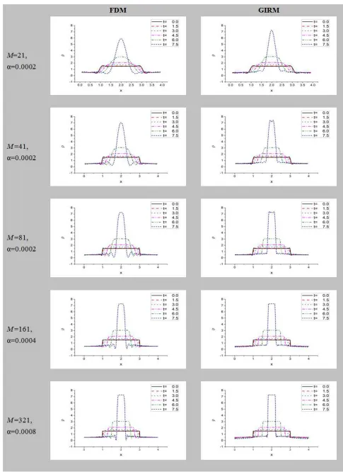
The parameters for numerical calculations are as follows:

4

=

L ; M=21,41,81161,321; dx=L M; γ =dx; 0025

. 0 =

dt ; T =3000dt; G=0.0015; ν =0; 0008 . 0 , 0004 . 0 , 0002 . 0 , 0 = α , (26)

where M , dx ,

γ

,

dt

and α are the number of

division of region 0<x<L, length of element, scale of G~, time interval and artificial damping coefficient. The

numerical solution is obtained for 0≤t≤T . The artificial

damping is given by adding 2 2

x

∂ ∂ ρ

α and 2 2

x u ∂

∂

(4)

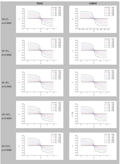
ρ and u, respectively, at every step of time evolution [6].

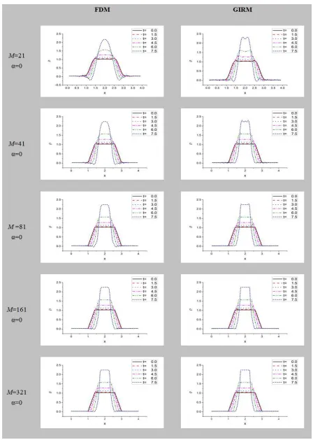
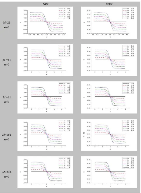
Distributions of density ρ and velocity u due to the

initial trapezoidal distribution of ρ are shown in Figs. 1a

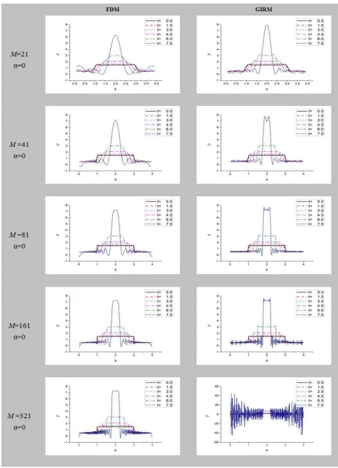
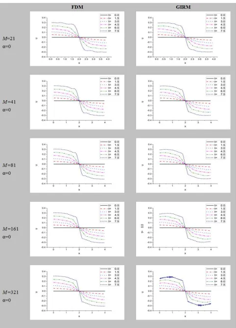
and 1b, respectively. Those due to the initial rectangular

distribution of ρ are shown in Figs. 2a and 2b, respectively.

Effects of artificial damping α on density ρ and velocity u

due to initial rectangular distribution of ρ are shown in Figs.

3a and 3b, respectively. FDM and GIRM give similar numerical results. However, if we observe the tendency of

density ρ as M increases, GIRM calculations give more

reasonable shape of density distribution. This suggests the

accuracy of GIRM results is higher than that of FDM results.

3.1.2. Without pressure and with Viscosity

4

=

L ; M=41; dx=L M_;γ =dx; dt=0.0025;

dt

T =3500,4000,5000 ; G=0.001,0.0015,0.002; 01

. 0 =

ν ; α =0, (27)

where ν is kinematic viscosity.

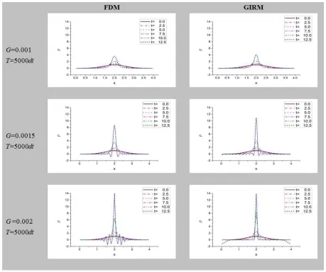
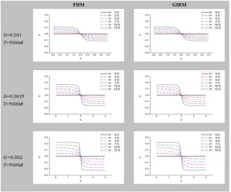
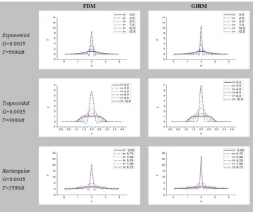
Effects of gravity G on density ρ and velocity u in case of

exponential initial distribution of ρ are shown in Figs. 4a and

4b. Comparisons among various distributions are given in Figs. 5a and 5b. FDM and GIRM give similar numerical

results. However, GIRM calculations give sharper

concentration of density ρ. This suggests the accuracy of

GIRM results is higher than those of FDM results.

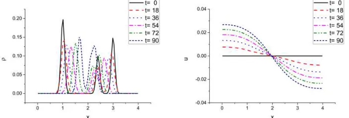
3.1.3. Merge of Multiple Lumps of Gas or Particles

We study a case where multiple lump of gas or particles

exist at time t=0:

∑

−

= 

   

  

      ₋ − = 1

0

2

exp )

0 , (

N

i i

x M

x

δ ξ

ρ , 0≤x≤L, (28)

where Mi, ξi and δi are mass, location and scale of a

lump of gas or particles. The lumps separated initially shorten the mutual distances and merge into a lump under the gravitational force.

4 =

L ; M=81; dx=L M; γ =dx; dt=0.0025; dt

T=30000 ; G=0.001; ν =0.03; α_ρ =0.0002_;

0 = vel

α ; N=3; M0=0.2; M1=0.1; M2=0.15;

L 25 . 0

0=

ξ ; ξ1=0.6L; ξ2=0.75L;

(29)

L L,0.05 025 . 0

0=

δ ; δ1=0.025L,0.05L;

L L,0.05 025 . 0

2=

δ ;

Numerical results are shown in Figs. 6 and 7. In Figs. 6

and 7, three lumps of gas or particles at t=0 merge into

two and one lumps under gravitational force, respectively. If

we continue the calculation, the two lumps at t=90 in Fig.

6 will merge into one lump.

3.2. Non-Zero Initial Velocity

Now, we study the case where the initial velocity is not zero:

1 5 . 0 exp 1

2 )

0 ,

( −

   



 ₋

− + =

L L x x

u

λ

, 0≤x≤L. (30)

Half of the first term on the right hand side is called Sigmoid

function. Sigmoid function is zero at

x

=

0 .

5 L

, and it tends

to zero and one when

x

tends to

+

∞

and

−

∞

,

respectively. The initial velocity distribution like this may correspond to the velocity distribution after big bang of cosmos or explosion of a star. However, in one- and two-dimensional gravity fields, we need infinite energy to move a particle from finite position to infinity. Hence, the fluid can’t expand to infinity against gravity. This is quite different from three-dimensional case.

The initial density distribution is an exponential one:

L x L

L x

x _ ≤ ≤

  

  

   

  ₋

−

= 0

05 . 0

5 . 0 exp

) 0 , (

2

ρ . (31)

14 =

L ; M =80,160,640; dx=L M ; γ =dx; 0025

. 0 =

dt ; T =2000dt; 04

. 0 , 02 . 0 , 01 . 0 , 0 =

G ; ν=0,0.02; 0048

. 0 , 0032 . 0 , 0016 . 0 , 0008 . 0 , 0 =

α . (32)

3.2.1. Case When Initial Velocity Distribution is Mild (λ=0.05)

GIRM results in case of mild initial velocity distribution

( λ=0.05 ) are shown in Fig. 8. The initial velocity

distribution is shown in, for example, Fig. 8(a). In case of mild initial velocity distribution, the fluid spreads to infinity

when G is zero. However, the fluid continue to concentrate

as far as the calculation converges when G is positive.

(5)

(6)

(7)

(8)

(9)

(10)

(11)

Figure 4a. Effects of gravity G on density ρ in case of exponential initial distribution of ρ.

3.2.2. Case When Initial Velocity Distribution is Moderate (λ=0.01)

GIRM results in case of moderate initial velocity

distribution (λ=0.01) are shown in Fig. 9. The initial

velocity distribution is shown in, for example, Fig. 9(a). In case of moderate initial velocity distribution, the fluid spreads first and then shrinks backward. Finally, the calculation diverges before the fluid region comes back to the origin.

3.2.3. Case When Initial Velocity Distribution is Radical (λ=0.002)

GIRM results in case of radical initial velocity distribution

(λ=0.002) are shown in Fig. 10. The initial velocity

distribution is shown in, for example, Fig. 10(a). In case of radical initial velocity distribution, the fluid spreads first and then shrinks backward rapidly. Finally, the calculation diverges before the fluid region comes back to the origin.

4. N

d

-Dimensional Fluid Motion without

Pressure

If xi, (i=1,2,⋯,Nd) and t refer to the coordinates

and time, the fluid motion in Nd-dimension is expressed as

0

= ∂ ∂ + ∂ ∂

i i

x u t

ρ ρ

, (33)

j j

i

i j i j i

x x

u x

x u u t u

∂ ∂

∂ + ∂

Π ∂ − = ∂ ∂ + ∂

∂ 2

ν , (34)

ρ πG x xi i

4

2

= ∂ ∂

Π ∂

(12)

Figure 4b. Effect of gravity G on velocity u in case of exponential initial distribution of ρ.

The summation convention is used for the repeated indices,

that is, 22 2 2

2 2 1 2 2

N i

i x x x x

x∂ =∂ ∂ +∂ ∂ + +∂ ∂

∂

∂ ⋯ . ui ,

) , , 2 , 1

(i= ⋯ Nd refers to the velocity vector. ρ, ν and

Π is the density, kinematic viscosity and gravitational

potential (Appendix A). G is the gravitational constant.

Since it’s not difficult to obtain two-dimensional expressions from three-dimensional ones, we develop theory using three-dimensional expressions below.

We rewrite the basic equations Eq. (34) as follows: Non-uniformity equation:

j i j i

x u

∂ ∂ =

θ . (36)

Constitutive equation:

j i j i

q =−νθ . (37) Equilibrium equation:

j j i

i j i j i

x q x u

t u

∂ ∂ − ∂

Π ∂ − = + ∂

∂ _θ

. (38)

We introduce Gaussian type Generalized Fundamental Solution (GFM) G~(x,ξ) with scale γi , (i=1,2,⋯,Nd) [4,5]:

∏

= 

   

 

 ₋

− = Nd

i i

i

x G

1

2 2

2 ) ( exp 2

1 )

, ( ~

γ ξ γ

π

ξ

x , (39)

(13)

Figure 5a. Comparisons of density ρ among various initial distributions of ρ.

i i i i x G t u t G x t u t ∂ ∂ = ∂ ∂ ( , ) ( , )~( , ) ) , ( ~ ) , ( ) ,

( x x xξ

ξ x x x ρ ρ i i x G t u t ∂ ∂ −ρ(x, ) (x, ) ~(x,ξ)

) , ( ~ ) , ( ) , ( ) , ( ~ ) , ( ) , ( ξ x x x ξ x x x i i i i t u t x G t u

t _ρ _δ

ρ ₋

∂ ∂

= , (40)

where ) , ( ~ ) , ( ~ ξ x ξ x i i x

G ₌_δ

∂ ∂

. (41)

integrating in region V , we obtain

∫∫∫

      ∂ ∂ + ∂ ∂ = V i i dV G x t u t t t x ξ x x x x ) , ( ~ ) , ( ) , ( ) , (

0 ρ ρ

∫∫∫

          − ∂ ∂ + ∂ ∂ = V i i i i dV t u t x G t u t t t G x ξ x x x ξ x x x x ξ x ) , ( ~ ) , ( ) , ( ) , ( ~ ) , ( ) , ( ) , ( ) , ( ~ δ ρ ρ ρ

∫∫

∫∫∫

+ ∂ ∂ =

S i i

V _t dV t u t G n dS

t

G x x x xξ x x

x ξ

x, ) ( , ) ( , ) ( , )~( , ) (

~ ρ _ρ

∫∫∫

−

V xt ui xt i(x,ξ)dVx

~ ) , ( ) , ( δ

ρ , (42)

where Sx and nxi are the boundary surface of V and the

unit outward normal to Sx, respectively. If we rewrite Eq.

(42), then, we have

∫∫∫

=

∂ ∂

V i i

V _t dV t u t dV

t

G x x x xξ x

x ξ

x, ) ( ,) ( , ) ( , )~( , ) (

~ ρ _ρ _δ

∫∫

−

S xt ui xt G(x,ξ)nxidSx

~ ) , ( ) , (

ρ . (43)

Exchanging

x

and

ξ

in Eq. (43), we obtain a generalized

integral representation for Eq. (33):

∫∫∫

=

∂ ∂

V i i

V _t dV t u t dV

t

G ξ ξ ξ ξx ξ

ξ x

ξ, ) ( , ) ( , ) ( , )~( , ) ( ~ δ ρ ρ

∫∫

−

S ξt ui ξt G(ξ,x)nξidSξ

~ ) , ( ) , (

ρ . (44)

Now, we obtain an integral representation of the equation of motion given by Eq. (34). From Eq. (41), we have

) , ( ~ ) , ( ) , ( ~ ) , ( ) , ( ~ ) , ( ξ x x ξ x x ξ x x j i j i j i t u x G t u G x t u _δ − ∂ ∂ = ∂ ∂

(14)

Figure 5b. Comparisons of velocity u among various initial distributions of ρ.

Figure 6. Merge of three lumps of gas or particles under gravity (GIRM, δ0=δ1=δ2=0.1).

Figure 7. Merge of three lumps of gas or particles under gravity (GIRM, δ0=δ1=δ2=0.2).

Multiplying G~(x,ξ) on the both sides of Eq. (36), we obtain

∫∫∫

   

   

∂ ∂ − =

V

j i j

i G dV

x t u

t xξ x

x

x, ) ( , ) ~( , ) (

0 θ

∫∫∫

   

 

   

 

+

∂ ∂ − =

V

j i

j i j

i

dV t

u

x G t u t G

x

ξ x x

ξ x x x

ξ x

) , ( ~ ) , (

) , ( ~ ) , ( ) , ( ) , ( ~

(15)

[

]

∫∫∫

+

=

V Gxξ ij xt ui xt j(x,ξ)dVx

~ ) , ( ) , ( ) , (

~ _θ _δ

∫∫

−

Sui xt G(x,ξ)nxjdSx

~ ) ,

( . (46)

Rewriting Eq. (46), we have

∫∫∫

=−

V i j

VG xξ ij xt dVx u xt G(x,ξ)dVx

~ ~ ) , ( ) , ( ) , (

~ _θ _δ

∫∫

+

Sui xt G(x,ξ)nxjdSx

~ ) ,

( . (47)

Exchanging x and ξ in Eq. (47), we obtain a generalized

integral representation for Eq. (36):

∫∫∫

=−

V i j

VG ξx ij ξt dVξ u ξt (ξ,x)dVξ

~ ) , ( ) , ( ) , (

~ _θ _δ

∫∫

+

SG(ξ,x)ui(ξ,t)nξjdSξ

~

. (48)

The generalized integral representation of Eq. (38) is obtained similarly. From Eq. (41), we have

) , ( ~ ) , ( ) , ( ~ ) , ( ) , ( ~ ) , ( ξ x x ξ x x ξ x x j j i j j i j j i t q x G t q G x t q δ − ∂ ∂ = ∂ ∂ . (49)

integrating in region V , we obtain

Figure 8. GIRM results (Mild initial velocity distribution).

∫∫∫

            ∂ ∂ + ∂ Π ∂ + + ∂ ∂ = V j j i i j i j i dV x t q x t t t u t t u

G _x x

x x x x ξ x ) , ( ) , ( ) , ( ) , ( ) , ( ) , ( ~ 0 θ

∫∫∫

            ∂ Π ∂ + + ∂ ∂ = V i j i j i dV x t G t t u G t t u G x x ξ x x x ξ x x ξ x ) , ( ) , ( ~ ) , ( ) , ( ) , ( ~ ) , ( ) , ( ~ θ

∫∫∫

_       − ∂ ∂ +

V ij j

j j i dV t q x t q G x ξ x x x ξ x ) , ( ~ ) , ( ) , ( ) , ( ~

δ

_∫∫∫

+

_∫∫∫

∂ ∂ =

V j ij

V

i _dV _G _u _t _t _dV

t t u

G~(x,ξ) (x, ) _x ~(x,ξ) (x, )θ (x, ) _x

∫∫∫

∂Π_∂

+ V i dV x t G x x ξ

x, ) ( , ) (

~

∫∫∫

∫∫

−

+

V ij j

SG xξqij xt njdSx q xt (x,ξ)dVx ~ ) , ( ) , ( ) , ( ~

(16)

Figure 9. GIRM results (Moderate initial velocity distribution)

Rewriting Eq. (50), we have

∫∫∫

=

∂ ∂

V ij j

V

i

dV t

q dV

t t u

G x x xξ x

x ξ

x, ) ( , ) ( , )~( , )

(

~ _δ ₋

_∫∫∫

VG(x,ξ)uj(x,t) ij(x,t)dVx

~ _θ

∫∫

∫∫∫

−

∂ Π ∂ −

S ij j

V

i

dS n t q G dV x

t

G~(x,ξ) (x, ) _x ~(x,ξ) (x, ) _x_{. (51)}

Exchanging x and ξ in Eq. (51), we obtain a generalized integral representation of Eq. (38):

∫∫∫

=

∂ ∂

V ij j

V

i

dV t

q dV

t t u

G ξ ξ ξx ξ

ξ x

ξ, ) ( , ) ( , )~( , ) (

~ _δ ₋

_∫∫∫

VG(ξ,x)uj(ξ,t) ij(ξ,t)dVξ

(17)

∫∫

∫∫∫

−

∂ Π ∂ −

S ij j

V

i

dS n t q G dV t

G ξ ξ x ξ ξ ξ

ξ x

ξ, ) ( , ) ~( , ) ( , ) (

~

ξ (52)

Figure 10. GIRM results (Radical initial velocity distribution).

) , (xt

Π and ∂Π(x,t) ∂xi are obtained by Eqs. (A17) or

(A10) in Appendix A in two- or three-dimension, respectively.

Then, we can obtain ρ(x,t) and ui(x,t) numerically, if we use the following process:

) , (x t

ρ and ui(x,t) are known

→

[∂ρ(x,t) ∂t

from Eq. (44)] and [θij(x,t) from Eq. (48)

→

) ,

( t

qij x from (37)

→

∂ui(x,t) ∂t from (52)]

→

ρ(x,t)from∂ρ(x,t) ∂t and ui(x,t+dt)

from ∂ui(x,t) ∂t

→

repeat. (53)

5. Numerical Results in Two-Dimension

(18)

dt t t y x t y x dt t y x ∂ ∂ + = + ) ( , , ) ( , , ) , ,

( ρ ρ

ρ , (54a)

dt t t y x u t y x u dt t y x u ∂ ∂ + = + ) ( , , ) ( , , ) , ,

( . (54b)

In FDM (Finite Difference Method) calculations, the central difference is used for the derivatives of unknown function f(x,t):

(

( , , ) ( , , )

)

2 1 ) , , ( t y dx x f t y dx x f dx x t y x f − − + ≈ ∂ ∂

, (55a)

(

( , , ) ( , , )

)

2 1 ) , , ( t dy y x f t dy y x f dy y t y x f − − + ≈ ∂ ∂

, (55b)

      − + − + ≈ ∂ ∂ ) , , ( ) , , ( 2 ) , , ( 1 ) , , ( 2 2 2 t y dx x f t y x f t y dx x f dx x t y x f

. (55c)

      − + − + ≈ ∂ ∂ ) , , ( ) , , ( 2 ) , , ( 1 ) , , ( 2 2 2 t dy y x f t y x f t dy y x f dy y t y x f

. (55d)

In GIRM (Generalized Integral Representation Method) calculations, the following approximations are used for the

weighted integral of unknown function f(x,t):

M L d

dx= ξ= , xi=ξi=−L+(i+0.5)dx (i=0,1,⋯,M−1), (56a)

N B d

dy= η= _, yj=µj=−B+(j+0.5)dy (j=0,1,⋯,N−1), (56b)

∫ ∫

₋L ₋ L

B

BG(ξ,η,x,y)f(ξ,η,t)dξdη ~

∑∑∫

−

∫

= − = + − + − ≈ 1 0 1 0 2 2 2

2 ( , , , ) ( , , )

~ M m N n n m d m d m d n d n t f d d y x

Gξ η ξ η ξ η

ξ ξ ξ ξ η η η

η , (56c)

∫

₋+ 2

∫

₋+ 2

2

2 ( , , , )

~ ξ ξ ξ ξ η η η

η ξ η ξ η

d m d m d n d

n G x y d d .

∑∑

= = _           + + − + + − ≈ 2 0 2 0 , , 3 ) 5 . 0 ( 2 , 3 ) 5 . 0 ( 2 ~

9 q p

n m y x d q d d p d G d d η η η ξ ξ ξ η ξ

. (56d)

∫ ∫

₋L ₋ ∂Π_∂ L B B i d d t y x

G ξ η

ξ η

ξ, , , ) ( , ) ( ~ ξ

∑∑∫

−

∫

= − = + − + − Π ≈ 1 0 1 0 2 2 2

2 ( , , , ) ( , , )

~ M m N n n m i d m d m d n d n t d d y x

Gξ η ξ η _ξ ξ η

ξ ξ ξ ξ η η η η

∑ ∑ ∫

+

∫

− = + − = + − + − Π ≈ 3 3 3 3 2 2 2

2 ( , , , ) ( , , )

~ i i m j j n n m i d m d m d n d n t d d y x

Gξη ξ η _ξ ξ η

ξ ξ ξ ξ η η η

η . (56e)

Eq. (56e) is very important to reduce the computational time.

First, we study the case where the initial velocity is zero:

0 ) 0 , , ( ) 0 ,

( =u x y =

u x _, −L≤x≤L & −L≤y≤L, (57)

where the infinite space is approximated by a computational

region −L≤x≤L & −L≤y≤L. In this case, the widely

distributed fluid continues to concentrate because of the gravitational attraction. This may correspond to aggregation of particles or gas in space.

5.1.1. Single Lump of Gas or Particles

Let’s assume a single lump of gas or particles. We consider two kinds of initial density distributions.

Exponential distribution: L r L L r y

x _ − ≤ ≤

            − = 2 4 . 0 exp ) 0 , , (

ρ , (58)

where r= x2+y2 .

Rectangular distribution:    ≤ < ≤ = r L L r y x 5 . 0 0 5 . 0 0 1 ) 0 , , (

ρ . (59)

An initial filter to reduce the numerical noise due to the discontinuity of the initial density distribution is defined as

      + − + − + + + + ) 0 , , ( 4 ) 0 , , ( ) 0 , , ( ) 0 , , ( ) 0 , , ( 8 1 y x dy y x y dx x dy y x y dx x ρ ρ ρ ρ ρ

. (60)

4

= =B

L ; M =N=21,41; dx=L M; dy=L N;

dx

=

1

γ ; γ2=dy; dt=0.0025; T =400dt,600dt;

1 . 0 =

G ; ν =0; α_ρ =0; αvel =0; off

on,

_flt=

(19)

Figure 11. Convergence tendency of FDM calculation (Exponential distribution)

Convergence tendency of FDM and GIRM solutions is shown in Figs. 11 and 12, respectively. Effects of the initial filter are shown in Figs. 13, 14, 15 and 16. We study the performance of the initial filter given by Eq. (60). The initial filter was applied to the rectangular density distribution given by Eq. (59). The results are shown in Figs. 13 and 14 in case

when M=N=21 and in Figs. 15 and 16 in case when M=N=41.

When the filters are applied to GIRM, the numerical noise due to discontinuity of initial density distribution is reduced sufficiently without damaging the accuracy.

5.1.2. Merge of Multiple Lumps of Gas or Particles

Let’s assume multiple lumps of gas or particles. We consider the following initial density distribution:

    

  

     

−

      − − =

2 2

15 . 0 15 . 0

2 . 0 exp ) 0 , , (

L y L

L x y

x

ρ _

  

  

     

−

    

 +

− +

2 2

15 . 0 15 . 0

2 . 0 exp 75 . 0

L y L

L x

L r L≤ ≤

− , (62)

(20)

Figure 12. Convergence tendency of GIRM calculation (Exponential distribution)

8 = =B

L ; M =N=41; dx=L M ; dy=L N;

dx

5 . 0

1=

γ ; γ2=0.5dy; dt=0.0025; T =2000dt;

1 . 0 =

G ; ν =2; αρ =0.016; αvel =0.016; off

_ flt=

ini ; (63)

In this examples, we used γ1=0.5dx and γ2 =0.5dy

instead of γ1=dx and γ2 =dy, since the former choice

gave slightly reasonable results than the latter choice. Numerical results are shown in Fig. 17. In Fig. 17, two

lumps of gas or particles at t=0 merge into one lump

under gravitational force.

5.2. Non-Zero Initial Velocity

Now, we study the case where the initial velocity is not zero:

r y x L

r v

u 1

5 . 0 1

. 0 exp 1 ) 0 , (

1

  

    

  



 

−

   

 

     

− + =

  

 

 −

x ,

L y L L x

L≤ ≤ − ≤ ≤

− & , (64)

where r= x2+y2. The infinite space is approximated by

L y L L x

L≤ ≤ − ≤ ≤

− & .

The initial density distribution is given by

    

  

     

−

     

− =

2 2

2 . 0 2

. 0 exp ) 0 , (

L y L

x x

ρ . (65)

4

= =B

L ; M=N=21; dx=2L M ; dy=2B N ;

dx

6 . 0

1=

γ ; γ2 =0.6dy; dt=0.0025; T =5000dt;

45 . 0 , 3 . 0 , 15 . 0 =

G ; ν =0.01; α_ρ=0, ; αvel =0, ; off

_flt=

ini ; (66)

In this examples, we used γ1=0.6dx and γ2=0.6dy

instead of γ1=dx and γ2 =dy, since the former choice

gave slightly reasonable results than the latter choice.

The numerical results are given in Figs. 18, 19 and 20 for

G=0.15, G=0.3 and G=0.45, respectively. In two-dimensional

gravity field too, we need infinite energy to move a particle from finite position to infinity as in one-dimensional gravity field. Hence, the fluid can’t expand to infinity against gravity. This is quite different from three-dimensional case. As is shown in the numerical examples, the fluid tries to spread first and then comes back to the origin. As the gravity increases, the fluid comes back rapidly. In Fig. 20, density

) , 0 ,

(x t

ρ at t=12.5 includes a spurious oscillation. If

21

=

M and N=21 are increased to

M

=

41

and

41 =

(21)

Figure 13. Effects of initial filter on density ρ on y=0 (Rectangular distribution).

(22)

Figure 15. Effects of initial filter on density ρ on y=0 (Rectangular distribution).

Figure 16. Effects of initial filter on velocity u on y=0 (Rectangular distribution).

(23)

Figure 18. Spreading and coming back of fluid (G=0.015, GIRM results).

6. Conclusions

In the present paper, application of Generalized Integral Representation Method (GIRM) to fluid dynamic motion of gas or particles in cosmic space was discussed. Spreading and merging or gas or particles under gravitational force was discussed through numerical calculations, and interesting results were obtained. Using one- and two-dimensional theory, merging of lumps of gas or particles was discussed. The effects of initial velocity field were also discussed. In contrast to three-dimensional theory, the fluid can’t spread to infinity in one- and two-dimensional theory. This means the importance of three-dimensional theory. Merging and spreading of gas or particles may be treated by the fluid dynamic approach, though we may need very big computational power and vast amount of time to obtain realistic numerical results in three-dimensional space.

In the present theory, although viscosity was included, pressure was neglected. For further discussion, introduction

of pressure and change of internal state of substance would be necessary. We studied one- and two-dimensional problems in the present paper. However, the real cosmic space is three

dimensional. Before challenging three dimensional

calculations, we need to study more to improve accuracy, stability and to reduce computational time [7].

Appendix A. Gravitational Potential

A.1. Newton’s law in three-dimensional space:

Force F12 acting on particles 1 and 2 with mass m1 and 2

m , respectively, is given by

| |

) (

2 1

2 1 2 1 12

x x

x x F

− − −

= Gmm , (A1)

where x1 and x2 are the position vectors of the particles 1

(24)

2 2 1 2 2 1 2 2 1 2

1 | ( ) ( ) ( )

|x −x = x −x + y −y + z −z . (A2)

The force field FU of a unit mass at the origin of the

coordinates is given by

3 2 1 2 1 | | ) ( x x x x F − − − = G

U . (A3)

The potential ΠU of three-dimensional gravitational field of

a unit mass at the origin of the coordinates is defined as

U U =−∇Π

F . (A4)

Hence, we obtain

r r r r F d r G d r G d U

U ⋅

     ∇ − = ⋅ = ⋅ − =

Π

_∫

3

_∫

1

r G r

Gd 1=− 1

     −

=

_∫

, (A5)

where r is |x|= x2+y2+z2 , and ΠU is assumed to

tend to 0 as r tends to infinity. If we use Gauss integral theorem

∫∫∫

−      ∂ ∂ + ∂ ∂ + ∂ ∂ ) ( 2 2 2 2 2 2 r

V _r dxdydz

G z y x G d d r r r G r

S sinθ θ φ 4π

1 ) ( 2 ₌ ∂ ∂ − =

_∫∫

∫∫∫

=4πG δ(x)δ(y)δ(z)dxdydz, (A6)

we have for the gravitational potential ΠU of a unit mass

given by Eq. (A5) satisfies

) ( ) ( ) ( 4 2 2 2 2 2 2 z y x G z y x U U

U = π δ δ δ

∂ Π ∂ + ∂ Π ∂ + ∂ Π ∂

. (A7)

Hence, the potential Πρ of the density distribution ρ:

x x x x _′ ′ − ′ − =

Π G

_∫∫∫

d

| |

) (

ρ

ρ (A8)

satisfies

ρ π

ρ 4 G

2_Π ₌

∇ . (A9)

The potential Πi and the force field Fi at x=xi due to mass mj (j=0,1,2,⋯,i−1,i+1,⋯,N−1) are given by

∑

≠ − − = Π i

j i j

j i

m G

|

|x x , (A10a)

∑

≠ − − − = Π −∇ = i

j i j

j i j i i i m G ₃ | | ) ( x x x x

F x , (A10b)

where 2 2 2 ) ( ) ( ) ( |

|xi−xj = xi−xj + yi−yj + zi−zj . (A11)

A.2. Newton’s Law in Two-Dimensional Space

The potential ΠU of two-dimensional gravitational field

of a unit mass at the origin of the coordinates is defined as

z d z z y x G y x U

U = − ′ ′

∂ Π ∂ + ∂ Π ∂

∫

₋+_∞∞ ( ) ) ( ) ( 4 2 2 2 2 δ δ δ π ) ( ) (

4πGδ xδ y

= . (A12)

Since π θ 2 ln ln ) ( ) ( 2 2 2 2 = ∂ ∂ =       ∂ ∂ + ∂ ∂

∫

∫∫

Sr Cr _r rd

r dxdy

r y

x , (A13)

where r=|x|= x2+y2 , the potential of two-dimensional

gravitational field due to a unit mass at the origin of coordinates is given by

r G

U =2 ln

Π . (A14)

Hence, the potential Π_ρ of the density distribution ρ

∫∫

′ − ′ ′ =

Π_ρ 2G ρ(x)ln|x x|dx (A15)

satisfies

ρ π

ρ 4 G

2_Π ₌

∇ . (A16)

The potential Πi and the force field Fi at x=xi due to

mass mj ( j=0,1,2,⋯,i−1,i+1,⋯,N−1) are given by

∑

≠ − = Π i j j i j

i 2G m lnr , (A17a)

∑

≠ − − − = Π −∇ = i

j i j

j i j i i i m G ₂ | | ) ( 2 x x x x

F x , (A17b)

where 2 2 ) ( ) ( |

|xi−xj = xi−xj + yi−yj . (A18)

A.3. Newton’s Law in One-Dimensional Space

The potential ΠU of one-dimensional gravitational field

of a unit mass at the origin of the coordinates is defined as

) ( 4 ) ( ) ( 4 2 2 x G y d y y x G dx

d ΠU = π δ

∫

+∞δ − ′ ′= π δ

∞

(25)

Since

2 | | |

|

2 2

=

     

=

    

 +

− +

−

∫

x

x x

x _dx

x d dx x dx

d

, (A20)

the potential of one-dimensional gravitational field due to a unit mass at the origin of coordinates is given by

| |

2 G x

U = π

Π . (A21)

Hence, the potential Πρ of the density distribution ρ:

∫∫

′ − ′ ′ =

Π_ρ 2πG ρ(x)|x x|dx (A22)

satisfies

ρ πG dx

d U

4

2 2

= Π

. (A23)

The potential Πi and the force field Fi at x=xi due to mass mj (j=0,1,2,⋯,i−1,i+1,⋯,N−1) are given by

∑

≠

− =

Π

i j

j i j

i 2πG m |x x |_{, (A24a)}

∑

≠ −

− =

Π −∇ =

i

j i j

j i j i

i x i

x x

x x m G F

| |

2π . (A24b)

References

[1] S. S. Kamisov, Cosmology

http://www1.maths.leeds.ac.uk/~serguei/teaching/cosmology.p df

[2] Lauro Moscardini and Klaus Dolag, Cosmology with

numerical simulations,

http://icc.ub.edu/~liciaverde/IC/como.pdf

[3] Gustavo Yepes, Cosmological Simulations of the Universe

And the Computational Challenges,

http://www.clues-project.org/talks/esac_grid_public.pdf [4] H. Isshik, S. Nagata, Y. Imai, “Solution of a diffusion problem

in a non-homogeneous flow and diffusion field by the integral representation method (IRM)”, Applied and Computational Mathematics, 3(1), (2014), pp. 15-26. http://article.sciencepublishinggroup.com/pdf/10.11648.j.acm. 20140301.13.pdf

[5] H. Isshiki, Theory and application of the generalized integral representation method (GIRM) in advection diffusion problem, Applied and Computational Mathematics, 3(4), (2014), pp. 137-149.

http://article.sciencepublishinggroup.com/pdf/10.11648.j.acm. 20140304.15.pdf

[6] H. Isshiki, A method for Reduction of Spurious or Numerical Oscillations in Integration of Unsteady Boundary Value Problem, AJET, 2, 3, (2014), pp. 190-202. file:///C:/Users/l/Downloads/1360-5725-2-PB%20(2).pdf [7] H. Isshiki, “Improvement of Stability and Accuracy of

Time-Evolution Equation by Implicit Integration”, Asian Journal of Engineering and Technology (AJET), Vol. 2, No. 2

(2014), pp. 1339–160.