Accelerating t-SNE using Tree-Based Algorithms
Laurens van der Maaten [email protected]
Pattern Recognition and Bioinformatics Group Delft University of Technology
Mekelweg 4, 2628 CD Delft, The Netherlands
Editors:Aaron Courville, Rob Fergus, and Christopher Manning
Abstract
The paper investigates the acceleration of t-SNE—an embedding technique that is com-monly used for the visualization of high-dimensional data in scatter plots—using two tree-based algorithms. In particular, the paper develops variants of the Barnes-Hut algorithm and of the dual-tree algorithm that approximate the gradient used for learning t-SNE em-beddings inO(NlogN). Our experiments show that the resulting algorithms substantially accelerate t-SNE, and that they make it possible to learn embeddings of data sets with millions of objects. Somewhat counterintuitively, the Barnes-Hut variant of t-SNE appears to outperform the dual-tree variant.
Keywords: embedding, multidimensional scaling, t-SNE, space-partitioning trees, Barnes-Hut algorithm, dual-tree algorithm.
1. Introduction
A plethora of embedding techniques have been proposed over the last decade, e.g., by Carreira-Perpi˜n´an (2010); Lawrence (2011); Roweis and Saul (2000); Tenenbaum et al. (2000); Saul et al. (2006); and van der Maaten and Hinton (2008). Reviews of these meth-ods are given by, e.g., van der Maaten et al. (2009) and Burges (2010). Because in high-dimensional spaces, only small pairwise distances are reliable, most of these techniques only try to accurately model such small pairwise distances in the low-dimensional embedding. In particular, a family of techniques that preserves small pairwise distances via stochas-tic neighbor embedding (SNE; Hinton and Roweis, 2003) has recently gained popularity (Carreira-Perpi˜n´an, 2010; van der Maaten and Hinton, 2008; Venna et al., 2010). Stochas-tic neighbor embedding techniques compute anN×N similarity matrix in both the original data space and in the low-dimensional embedding space in such a way, that the similarities form a probability distribution over pairs of objects. The distribution over pairs of objects is defined such that pairs of similar objects have a high probability under the distribution, whilst pairs of dissimilar points have a low probability. Specifically, the probabilities are generally given by a normalized Gaussian or Student-t kernel computed from the input data or from the embedding. The low-dimensional embedding is learned by minimizing the Kullback-Leibler divergence between the two probability distributions (computed in the original data space and the embedding space) with respect to the locations of the points in the embedding. Because of the asymmetry of the Kullback-Leibler divergence, stochas-tic neighbor embedding focuses on accurately modeling small pairwise distances, i.e., on preserving local data structure in the low-dimensional embedding.
Because the objective functions of most stochastic neighbor embedding techniques are non-convex,1 the minimization of the objective is typically performed using first-order or second-order gradient-descent techniques (Carreira-Perpi˜n´an, 2010; Hinton and Roweis, 2003; Vladymyrov and Carreira-Perpi˜n´an, 2012). The gradient of the Kullback-Leibler divergence that is minimized has a very natural interpretation as an N-body system in which all of theN points in the low-dimensional embedding exert forces on each other, and the resultant force on each of the points needs to be computed.
Because the computation of stochastic neighbor embedding gradients involves the eval-uation of forces between allN×N pairs of points, one of the main limitations of stochastic neighbor embedding is that its computational complexity scales quadratically in the num-ber of input objects N. In practice, this limits the applicability of stochastic neighbor embedding to data sets with only a few thousand points. To visualize larger data sets, landmark implementations of stochastic neighbor embedding may be used (van der Maaten and Hinton, 2008), but this is hardly a satisfactory solution because it does not facilitate visualization of all available data. Alternatively, computational problems may be circum-vented by learning a parametric function between the input space and the embedding using a type of stochastic gradient descent (van der Maaten, 2009), but such an approach sub-stantially complicates learning and is only applicable when the input data takes the form of high-dimensional data vectors.
In this paper, we explore tree-based approaches for stochastic neighbor embedding that require onlyO(NlogN) computation andO(N) memory. Our approaches compute a sparse
approximation of the similarities between the input objects using vantage-point trees (Yian-ilos, 1993), and subsequently, they approximate the forces between the points in the embed-ding with the help of either a Barnes-Hut algorithm (Barnes and Hut, 1986) or a dutree al-gorithm (Gray and Moore, 2001, 2003). The Barnes-Hut and dual-tree alal-gorithms reduce the number of pairwise forces that needs to be computed by exploiting the fact that the forces exerted between two small groups of points are all very similar whenever these two groups are relatively far away. We will study the performance of the tree-based algorithms in the con-text of the successful t-distributed stochastic neighbor embedding (t-SNE; van der Maaten and Hinton, 2008) algorithm, but similar computational approaches may be used to speed up, e.g., standard stochastic neighbor embedding (Hinton and Roweis, 2003), the neigh-borhood retrieval visualizer (NeRV; Venna et al., 2010), and elastic embedding (Carreira-Perpi˜n´an, 2010; Vladymyrov and Carreira-Perpi˜n´an, 2014). Source code of our tree-based t-SNE algorithms is publicly available onhttp://homepage.tudelft.nl/19j49/tsne; this software has recently been successfully used to create large-scale embeddings of, among others, mouse brain data (Ji, 2013), metagenomic data (Laczny et al., 2014), and word embeddings (Cho et al., 2014). This paper is an extended version of an earlier conference publication (van der Maaten, 2013) on a Barnes-Hut approximation to t-SNE, which was recently independently investigated by Yang et al. (2013). Compared to these prior papers, this paper: (1) investigates a second tree-based algorithm to speed up t-SNE, viz. the dual-tree algorithm, whereas van der Maaten (2013) and Yang et al. (2013) only considered the Barnes-Hut algorithm; (2) contains more detailed explanations of the techniques and experiments; and (3) contains additional experimental results on a number of large data sets.
The outline of the remainder of this paper is as follows. In Section 2, we discuss related work on accelerating algorithms that scale quadratically in the data set size. Section 3 reviews the t-SNE algorithm of van der Maaten and Hinton (2008). In Section 4, we present accelerated variants of t-SNE that are based on the Barnes-Hut and on the dual-tree algorithm. Our experimental results are presented in Section 5. Section 6 concludes the paper and presents directions for future work.
2. Related Work
This work fits in a larger body of prior work that has focused on decreasing the com-putational complexity of algorithms that scale quadratically in the amount of data when implemented naively, such as nearest neighbor search and Parzen density estimation.
strong performance reported in earlier work by Liu et al. (2004), we opt to use metric trees to approximate the similarities of the input objects in our algorithms.
Prior work on accelerating N-body computations, e.g., to perform fast Parzen density estimation, is generally based onO(NlogN) tree-based algorithms such as the Barnes-Hut algorithm (Barnes and Hut, 1986) and the dual-tree algorithm (Gray and Moore, 2001, 2003), or on O(N) fast multipole methods (Rokhlin, 1985). We explain the Barnes-Hut and dual-tree algorithms in more detail in Section 4. Fast multipole methods perform ex-pansions of the forces that points exert on each other that are specific to the functional form of those forces, and use these expansions to speed up the computations (Rokhlin, 1985). For instance, if the strength of the interactions is governed by a Gaussian function, the interactions may be approximated by a weighted sum of Hermite polynomials: the interac-tion I(·,·) between objectsxand y then factorizes asI(x,y) =f(x)g(y), which facilitates the computation of all resultant forces in O(N). For Gaussian forces, the fast multipole approach is generally referred to as the fast Gauss transform (Greengard and Rokhlin, 1987; Yang et al., 2003). The aforementioned algorithms for fast N-body computations are commonly used in astronomy, e.g., for simulating large galaxies (Springel et al., 2001; Croton et al., 2006), and in information visualization, e.g., for constructing force-directed layouts and for graph drawing (Fruchterman and Reingold, 1991; Chalmers, 1996; Quigley and Eades, 2000; Hu, 2005). Lang et al. (2005) presents an experimental comparison of many of the algorithms.
In machine learning, dual-tree algorithms have been used for, among others, density estimation (Gray and Moore, 2001, 2003) and Gaussian process regression (Gray, 2004). Raykar and Duraiswami (2006) have used fast multipole methods to speed up Parzen density estimators. de Freitas et al. (2006) also used fast multipole approaches to speed up the computation of GaussianN-body interactions, in particular, in order to speed up generalized eigenvalue solvers based on Krylov subspace iteration as well as to speed up active learning (Mahdaviani et al., 2005) and stochastic neighbor embedding. Recently, Vladymyrov and Carreira-Perpi˜n´an (2014) have also explored a fast multipole approach for constructing embeddings, focusing on the elastic-embedding algorithm. Unfortunately, the fast multipole approach cannot be readily applied to t-SNE because, to the best of our knowledge, there exists no appropriate expansion for forces governed by Student-t interactions: using fast multipole methods for t-SNE would thus require further approximations that, for instance, replace the Student-t interactions in the learning gradient by Gaussian interactions.
3. t-Distributed Stochastic Neighbor Embedding
t-Distributed stochastic neighbor embedding (t-SNE) minimizes the divergence between two distributions: a distribution that measures pairwise similarities of the input objects and a distribution that measures pairwise similarities of the corresponding low-dimensional points in the embedding. Assume we are given a data set of (high-dimensional) input objectsD={x1,x2, . . . ,xN} and a functiond(xi,xj) that computes a distance between a
pair of objects, e.g., the Euclidean distanced(xi,xj) =kxi−xjk. Our aim is to learn ans
-dimensional embedding in which each object is represented by a point,E ={y1,y2, . . . ,yN}
withyi ∈Rs (typical values forsare 2 or 3). To this end, t-SNE defines joint probabilities
conditional probabilities
pj|i=
exp(−d(xi,xj)2/2σi2)
P
k6=iexp(−d(xi,xk)2/2σi2)
, pi|i = 0,
pij =
pj|i+pi|j
2N .
In the above equation, the bandwidth of the Gaussian kernels, σi, is set in such a way
that the perplexity of the conditional distribution Pi equals a predefined perplexity u. As
a result, the optimal value of σi varies per object: in regions of the data space with a
higher data density, σi tends to be smaller than in regions of the data space with lower
density. The optimal value of σi for each input object can be found using a simple binary
search (Hinton and Roweis, 2003) or using a robust root-finding method (Vladymyrov and Carreira-Perpi˜n´an, 2013).
In thes-dimensional embeddingE, the similarities between two pointsyiandyj(i.e., the
low-dimensional models ofxi andxj) are measured using a normalized heavy-tailed kernel.
Specifically, the embedding similarityqij between the two pointsyi and yj is computed as
a normalized Student-t kernel with a single degree of freedom
qij =
(1 +kyi−yjk2)−1
P
k6=l(1 +kyk−ylk2)−1
, qii= 0.
The heavy tails of the normalized Student-t kernel allow dissimilar input objects xi and
xj to be modeled by low-dimensional counterparts yi and yj that are too far apart. This
is desirable because it creates more space to accurately model the small pairwise distances (i.e., the local data structure) in the low-dimensional embedding.
The locations of the embedding points yi are determined by minimizing the
Kullback-Leibler divergence between the joint distributionsP and Q:
C(E) =KL(P||Q) =X
i6=j
pijlog
pij
qij
.
Due to the asymmetry of the Kullback-Leibler divergence, the objective function focuses on modeling high values of pij (similar objects) by high values of qij (nearby points in the
embedding space). The objective function is non-convex in the embeddingE. It is typically minimized by descending along the gradient
∂C ∂yi
= 4X
j6=i
(pij −qij)qijZ(yi−yj),
where we defined the normalization term Z =P
k6=l(1 +kyk−ylk2)
−1.
It is straightforward to see that the evaluation of the joint distributions P and Q is
4. Tree-Based Algorithms for t-SNE
We explore two fast algorithms to approximate the t-SNE gradient ∂∂Cy
i: (1) an algorithm
based on the Barnes-Hut approximation and (2) an algorithm based on the dual-tree approx-imation. Both variants use the same algorithm to approximate the similarities computed between the input data,viz. they use a metric tree to approximateP by a sparse distribu-tion in which onlyO(uN) values are non-zero. This approximation of the input similarities is described in detail in Section 4.1. The Barnes-Hut and dual-tree approximations are presented in Section 4.2 and 4.3, respectively.
4.1 Approximating Input Similarities
The input similarities in t-SNE are defined as normalized Gaussian kernel values. As a result, probabilities pij that correspond to dissimilar input objects i and j are nearly
in-finitesimal. Therefore, we can develop a sparse approximation for the probabilities pij
without negatively affecting the quality of the final embeddings. In particular, we compute the sparse approximation by finding the b3uc nearest neighbors of each of the N input objects (recall thatuis the perplexity of the conditional distributions), and we redefine the pairwise similarities between the input objects,pij, as
pj|i =
( exp(−d(xi,x
j)2/2σi2)
P
k∈Niexp(−d(xi,xk)2/2σ2i), ifj∈ Ni
0, otherwise
(1)
pij =
pj|i+pi|j
2N . (2)
Herein, Ni represents the set of the b3uc nearest neighbors of xi, and the bandwidth σi is
set such that the perplexity of the conditional distribution equals a predefined perplexityu
via a binary search overσi. The nearest neighbor setsNi are found inO(uNlogN) time by
building a vantage-point tree on the input data and performing an exact nearest-neighbor search with the help of the resulting tree.
In a vantage-point tree, each node stores an input object and the radius of a (hyper)ball that is centered on this object (Yianilos, 1993). All non-leaf nodes in the tree have two children: objects that are locatedinsidethe ball are stored under the left child of the node, whereas objects that are locatedoutsidethe ball are stored under the right child. The tree is constructed by presenting the objects one-by-one, traversing the tree based on whether the current object lies inside or outside a ball, and creating a new leaf node in which the object is stored. The radius of the new leaf node is set to the median distance between its object and all other objects that lie inside the ball represented by its parent node. To construct a vantage-point tree, the objects need not necessarily be points in a high-dimensional feature space; the availability of a metricd(xi,xj) suffices. Therefore, the use of vantage-point trees
facilitates the application of our algorithms even on complex data types, provided a metric
d(xi,xj) is available. In all our experiments, the input data comprises high-dimensional
vectors,xi ∈RD, and we use the metric d(xi,xj) =kxi−xjk.
the distance τ to the furthest nearest neighbor in the current neighbor list. The value of
τ determines whether or not a node should be explored: if there can still be objects inside the ball whose distance to the target object is smaller thanτ, the left node is searched, and if there can still be objects outside the ball whose distance to the target object is smaller than τ, the right node is searched. The order in which children are explored depends on whether or not the target object lies inside or outside the current node ball: the left child is examined first if the object lies inside the ball, because the odds are that the nearest neighbors of the target object are also located inside the ball. Conversely, the right child is examined first whenever the target object lies outside of the ball.
The nearest-neighbor search is performed for all N input objects in D in order to ob-tain the nearest-neighbor sets Ni. Afterwards, it is straightforward to compute the input similarities via Equation 1 and 2.
4.2 Barnes-Hut Approximation
To approximate the t-SNE gradient, we start by splitting the gradient into two parts
∂C ∂yi
= 4(Fattr+Frep) = 4
X
j6=i
pijqijZ(yi−yj)−
X
j6=i
q2ijZ(yi−yj)
, (3)
where Fattr denotes the sum of all attractive forces (the left sum), whereas Frep denotes
the sum of all repulsive forces (the right sum). Computing the sum of all attractive forces,
Fattr, is computationally efficient; it can be done by summing over all non-zero elements
of the sparse distribution P that was constructed using the procedure described in the previous subsection in O(uN).2 However, a naive computation of the sum of all repulsive forces, Frep, is still O(N2). We now develop a Barnes-Hut algorithm to approximateFrep
efficiently in O(NlogN).
Consider three points yi, yj, and yk with kyi−yjk ≈ kyi−ykk kyj −ykk. In this
situation, the contributions of yj and yk to Frep will be roughly equal. The Barnes-Hut
algorithm (Barnes and Hut, 1986) exploits this by (1) constructing a quadtree or octtree on the current embedding,3 (2) traversing the quadtree using a depth-first search, and (3) at every node in the quadtree, deciding whether the corresponding cell can be used as a “summary” for the contributions to Frep of all points in that cell.
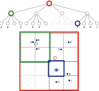
A quadtree is a tree in which each node represents a rectangular cell with a particular center, width, and height. Non-leaf nodes have four children that split up the cell into four smaller cells (quadrants) that lie “northwest”, “northeast”, “southwest”, and “southeast” of the center of the parent node; see Figure 1 for an illustration of a quadtree. Leaf nodes represent cells that contain at most one point of the embedding; the root node represents the cell that contains the complete embedding. In each node, we store the center-of-mass of the embedding points that are located inside the corresponding cell, ycell, and the total
number of points that lie inside the cell, Ncell. A quadtree has O(N) nodes and can be
constructed inO(N) time by inserting the points one-by-one, splitting a leaf node whenever
2. Note that the termqijZ= (1 +kyi−yjk2)−1 can be computed inO(1).
A B
C
D
E
F
G
H I
A B C D E F G H I
Figure 1: Illustration of a quadtree that was constructed on a data set of nine two-dimensional data points. The top half of the figure illustrates the structure of the tree that represents the partitioning of the two-dimensional space shown in the lower half of the figure. Corresponding colors are used to highlight corresponding elements of the graph and the space partitioning. Nodes in the graph correspond to square cells in the space (deeper nodes correspond to smaller cells). In each node, we store: (1) the number of points that are located in the corresponding cell and (2) the center-of-mass of those points (the centers-of-mass of the three highlighted cells are illustrated by the opaque circles in the space partitioning). The opaque parts of the tree are not actually created, because the corresponding parts of the space do not contain any data points. Leaf nodes represent cells that contain at most one data point. As a result, denser areas of the space correspond to parts of the tree that are deeper.
a second point is inserted in its cell, and updatingycell and Ncell of all visited nodes. Note
that the in denser regions of the embedding, the quadtree is deeper than in regions with sparse data.
To approximate the repulsive part of the gradient, Frep, we note that if a cell is
suffi-ciently small and suffisuffi-ciently far away from point yi, the contributions −q2ijZ(yi−yj) to
Frep will be roughly similar for all points yj inside that cell. We can, therefore,
points inside the cell, ycell represents the center-of-mass of the cell, and where we define
qi,cellZ = (1 +kyi −ycellk2)−1. This approximation is illustrated in Figure 2. We first
approximate FrepZ =−qij2Z2(yi−yj) by performing a depth-first search on the quadtree,
assessing at each node whether or not that node may be used as a “summary” for all the embedding points that are located in the corresponding cell. During this search, we also con-struct an estimate ofZ =P
i6=j(1 +kyi−yjk2)−1in the same way. The two approximations
thus obtained are then used to compute Frep via Frep = FrepZZ .
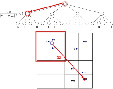
We use the condition proposed by Barnes and Hut (1986) to decide whether a cell may be used as a “summary” for all points in that cell. The condition compares the distance between the cell and the target point with the size of that cell by evaluating
rcell kyi−ycellk2
< θ, (4)
where rcell represents the length of the diagonal of the cell under consideration and θ
is a threshold that trades off speed and accuracy (higher values of θ lead to faster but coarser approximations). Note that when θ = 0, all pairwise interactions are computed, and the Barnes-Hut approximation reduces to naive computation of the t-SNE gradient. In preliminary experiments, we also explored various other conditions that take into account the rapid decay of the Student-t tail, but we did not find these alternative conditions to lead to a better accuracy-speed trade-off. The problem of more complex conditions is that they require expensive computations at each cell. By contrast, the condition in Equation 4 can be evaluated very rapidly.
4.3 Dual-tree Approximation
Whilst the Barnes-Hut algorithm considers point-cell interactions, further speed-ups may be obtained by computing only cell-cell interactions. This can be done using a dual-tree algorithm of Gray and Moore (2001). The dual-tree algorithm simultaneously traverses the same quadtree twice in a depth-first manner. For every pair of nodes, the dual-tree algorithm decides whether or not the interaction between the cells of quadtree A and quadtree B can be used as “summary” for the interactions between all points inside these two cells (note that quadtree A and B are identical trees). If the summary condition is passed, the corresponding force is computed. Subsequently, we perform the following additions: (1) we add to all children of the node under consideration in tree A the product of the force and the number of children in the relevant node of tree B; and (2) we add to all children of the node under consideration in tree B the product of the force and the number of children in the node of tree A. Subsequently, all children of the cells in quadtree A and B are pruned. In the dual-tree approximation, we check whether the interaction between a pair of nodes may be used as a “summary” interaction using the condition
max(rcell−A, rcell−B) kycell−A−ycell−Bk2
< θ,
where ycell−A and ycell−B represent the center-of-mass of the two cells from quadtree A
and B under consideration and where rcell−A and rcell−B represent the diameter of these
A B
C
D
E
F
G
H I
A B C D E F G H I
3x
rcellkyi ycellk2 < ✓
Figure 2: Illustration of the Barnes-Hut approximation. To evaluate the t-SNE gradient for point I, the Barnes-Hut algorithm performs a depth-first search on the embedding quadtree, checking at every node whether or not the node may be used as a “summary”. In the illustration, the cell containing points A, B, and C satisfies the summary-condition: the force between the center-of-mass of the three points (which is stored in the quadtree node) and point I is computed, multiplied by the number of points in the cell (i.e., by three), and added to the gradient for point I. All children of the summary node are pruned from the depth-first search.
exactly in dual-tree t-SNE. However, in dual-tree t-SNE, the dual-tree algorithm is used to compute the repulsive part, Frep, of the t-SNE gradient. Note that the optimal value for
θ generally differs between Barnes-Hut and dual-tree algorithms, because both algorithms summarize interactions differently.
those points (after multiplication with the appropriate number of children). Alternatively, we could construct and store a list of all children for each node during tree construction, but this is computationally equally costly and requires substantial additional memory.4
5. Experiments
We performed experiments on five large data sets to evaluate the performance of the Barnes-Hut and dual-tree variants of t-SNE. An implementation of the two algorithms (as well as an implementation of the original t-SNE algorithm) is available from http: //homepage.tudelft.nl/19j49/tsne. We describe the data sets we used in our experi-ments in Section 5.1. The setup of our experiexperi-ments is presented in Section 5.2, and the results of our experiments are presented in Section 5.3.
5.1 Data Sets
We performed experiments on five data sets: (1) the MNIST data set, (2) the CIFAR-10 data set, (3) the NORB data set, (4) the street view house numbers data set, and (5) the TIMIT data set. We briefly describe each of the five data sets as well as the preprocessing we applied on the data below.
MNIST.The MNIST data set containsN= 70,000 gray scale handwritten digit images of size D= 28×28 = 784 pixels (real-valued between 0 and 1), each of which corresponds to one of ten classes. We directly use the pixel values as input into our embedding algorithms without any further preprocessing.
CIFAR-10. The CIFAR-10 data set (Krizhevsky, 2009) is an annotated subset of the 80 million tiny images data set of Torralba et al. (2008) that contains N = 70,000 RGB images of size 32×32 pixels. Each image corresponds to one of ten classes. To extract features from the images, we trained a convolutional network with three convolutional layers on the training images using Caffe (Jia, 2013). We used a network with the following structure: (1) two convolutional layers that contain 32 filters of size 5×5, compute rectified linear unit (ReLU) activations, perform max-pooling over 3×3 patches, and perform local response normalization over 3×3 patches; (2) one convolutional layer with 64 filters of size 5×5, ReLU activations, and average pooling over 3×3 patches; and (3) a final fully connected layer followed by a softmax activation function. The weights of the network were randomly initialized by sampling from a Gaussian distribution with a small variance; all biases were initialized to zero. The network was trained to minimize cross-entropy loss with hundred full sweeps through the data using mini-batches of size 100, a slowly decaying learning rate, and a momentum term of 0.9. The network was regularized using standard (L2) weight decay, using λ= 0.004. The resulting network obtained a training error of 0.1087 and a test error of 0.1870 on the CIFAR-10 data set, which is on par with the performance of convolutional networks (without data augmentation) on this data set reported in prior studies (Krizhevsky, 2009; Hinton et al., 2012). We used the activations in the last convolutional layer (after the average pooling) asD= 1,024-dimensional features for the images. Please note that supervised information was used to obtain these features.
Computation time Nearest neighbor error
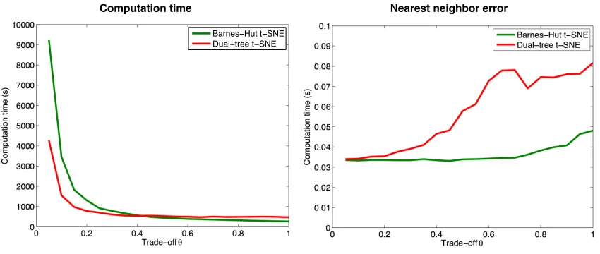
Figure 3: Computation time (in seconds) required to embed 70,000 MNIST digits using two accelerated variants of t-SNE (left) and the 1-nearest neighbor errors of the corresponding embeddings (right) as a function of the trade-off parameterθ. The green lines represent the performance of the Barnes-Hut approximation, whereas the red lines represent the performance of the dual-tree approximation. Note that the special caseθ= 0 corresponds to standard t-SNE.
NORB. The (small) NORB data set (LeCun et al., 2004) contains gray scale images of toys from five different classes, rendered on a uniform background under 6 lighting con-ditions, 9 elevations (30 to 70 degrees every 5 degrees), and 18 azimuths (0 to 340 every 20 degrees). All N= 48,600 images contain 96×96 = 9,216 pixels. We preprocess the images using a simple high-pass filter (specifically, a Laplacian-of-Gaussian filter with σ2= 1 pix-els) in order to remove low-frequency information such as the intensity value of the image background. This leads to feature representations of dimensionality D= 9,216, which were used as input into the embedding algorithms.
Computation time Nearest neighbor error
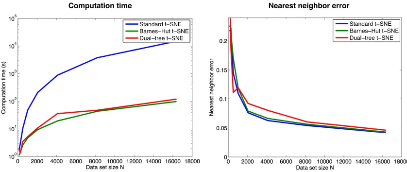
Figure 4: Computation time (in seconds) required to embed MNIST digits (left) and the 1-nearest neighbor errors of the corresponding embeddings (right) as a function of data set size N for standard t-SNE (in blue), Barnes-Hut t-SNE (in green), and dual-tree t-SNE (in red). Note that the required computation time, which is shown on they-axis of the left figure, is plotted on a logarithmic scale.
in the last convolutional layer as features for the house number images. Please note that supervised information was used to obtain these features.
TIMIT. The TIMIT data set contains 3,696 spoken utterances (with a total of N = 1,105,455 frames) by both male and female speakers.5 Each frame of the utterances is labeled according to one of 39 phones. The features that we used in our experiments are 13 mel-frequency cepstral coefficients (MFCC features) computed on sliding windows of speech with 25 ms windows at a 10 ms frame rate. In addition, we employ the corresponding delta features and delta-delta features (Sha and Saul, 2006), which leads to a 39-dimensional feature representation. For each frame, all MFCC features within a window of width 7 are concatenated, leading toD= 273-dimensional feature vectors that are used as input data.
5.2 Experimental Setup
In all experiments, we follow the experimental setup of van der Maaten and Hinton (2008) as closely as possible. In particular, we initialize the embedding E by sampling the points yi from a Gaussian with a variance of 10−4, and we run a gradient-descent optimizer for
1,000 iterations, setting the initial step size to 200. We update the step size during the optimization using the scheme of Jacobs (1988). We use an additional momentum term that has weight 0.5 during the first 250 iterations, and 0.8 afterwards. In all experiments, the perplexity u used to compute the input similarities is fixed to 50. All data sets were preprocessed using PCA to reduce their dimensionality to 50 before t-SNE was performed.
During the first 250 learning iterations, we multiplied all pij-values by a user-defined
constant α >1. As explained by van der Maaten and Hinton (2008), this trick enables t-SNE to find a better global structure in the early stages of the optimization by creating very tight clusters of points that can easily move around in the embedding space. In preliminary experiments, we found that this trick becomes increasingly important to obtain good embeddings when the data set size increases, as it becomes harder for the optimization to find a good global structure when there are more points in the embedding because there is less space for clusters to move around. In our experiments, we fix α= 12 (by contrast, van der Maaten and Hinton, 2008 used α= 4).
5.3 Results
We present the results of three sets of experiments. In the first experiment, we investigate the effect of the trade-off parameterθon the speed and the quality of embeddings produced by Barnes-Hut t-SNE and dual-tree t-SNE on the MNIST data set. In the second exper-iment, we investigate the computation time required by both approaches as a function of the number of input objects N (also on the MNIST data set). In the third experiment, we construct and visualize embeddings of all five data sets. All computation times were measured on a laptop computer with an Intel Core i5 4258U CPU running at 2.6GHz.
Experiment 1. Figure 3 presents the results of experiments with Barnes-Hut t-SNE and dual-tree t-SNE in which we varied the speed-accuracy trade-off parameter θ used to construct the embedding. The figure shows the computation time required to construct embeddings of all 70,000 MNIST digit images, as well as the 1-nearest neighbor error (com-puted based on the digit labels) of the corresponding embeddings. The nearest-neighbor error of an embedding is a measure for the quality of an embedding. Note that the special caseθ= 0 corresponds to standard t-SNE of van der Maaten and Hinton (2008); we did not perform an experiment withθ= 0 because standard t-SNE would take too long to complete on the full MNIST data set.
The results presented in the figure highlight the merits of using tree-based t-SNE algo-rithms. In particular, the results show that Barnes-Hut t-SNE with θ = 0.5 and dual-tree t-SNE with θ = 0.2 lead to embeddings that are of the same quality as those obtained with standard t-SNE (when quality is measured in terms of nearest-neighbor errors in the embedding). At the same time, increasing the value of θ to these values leads to very substantial improvements in terms of the amount of computation required to construct the embedding: for example, Barnes-Hut t-SNE requires only 751 seconds to embed all 70,000 MNIST digits whenθ= 0.5, whereas the original t-SNE algorithm would have taken many days to complete. The results presented in the figure also suggest that dual-tree t-SNE has a slightly worse speed-accuracy trade-off than Barnes-Hut t-SNE: Barnes-Hut t-SNE with
θ= 0.5 leads to an embedding of slightly higher quality than dual-tree t-SNE withθ= 0.2, whilst at the same time requiring fewer computational resources.
MNIST: 12m 31s
CIFAR-10: 13m 20s
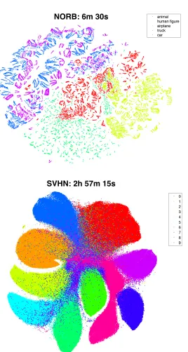
NORB: 6m 30s
SVHN: 2h 57m 15s
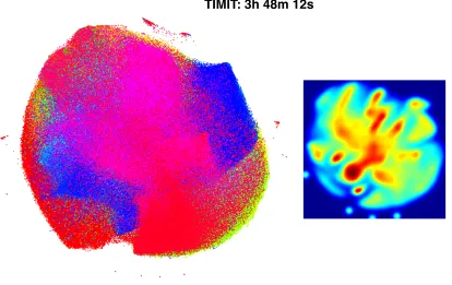
TIMIT: 3h 48m 12s
Figure 7: Barnes-Hut t-SNE visualization obtained with θ = 0.5 of the TIMIT speech frames data set. The left figure shows a scatter plot in which the colors of the points indicate the classes of the corresponding objects. The right figure shows a Parzen density estimate of the two-dimensional embedding. The title of the figure indicates the computation time that was used to construct the corresponding embeddings. Figure best viewed in color.
previous experiment 1, we fixed the parameterθto 0.5 in the experiments with Barnes-Hut t-SNE; in the experiments with dual-tree t-SNE, we fixedθ to 0.2.
The results presented in Figure 4 show that both Barnes-Hut SNE and dual-tree t-SNE are indeed orders of magnitude faster than standard t-t-SNE, whilst the difference in quality of the constructed embeddings (which is measured by the nearest-neighbor errors) is negligible. Most prominently, the computational advantages of Barnes-Hut t-SNE and dual-tree t-SNE rapidly increase as the number of objects in the data set N increases. The results also suggest that a fixed value of θ= 0.5 for Barnes-Hut t-SNE and θ= 0.2 for dual-tree t-SNE appears to work well across a range of data set sizes N. As in the first experiment, the results of this experiment also suggest that Barnes-Hut t-SNE slightly outperforms dual-tree t-SNE in terms of the trade-off between quality of the embedding and the associated computational costs.
corresponding objects; the titles of the plots indicate the computation time that was used to construct the corresponding embeddings.
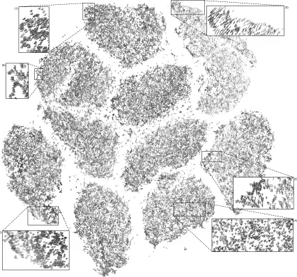
The visualization in the top part of Figure 5 shows that Barnes-Hut t-SNE can effi-ciently construct high-quality embeddings of the 70,000 MNIST handwritten digit images: although no supervised information was used, all ten digit classes are clearly separated in an embedding that was constructed in just over 12 minutes. Although our MNIST embedding contains many more points, it may be compared with that presented by van der Maaten and Hinton (2008). Visually, the structure of the two embeddings is very similar.
The results on the CIFAR-10 data set (in the bottom part of Figure 5) show a reasonably good separation of classes; in particular, classes such astruck andship are clearly separated from the other classes. To evaluate the quality of the CIFAR-10 embedding, we measured the generalization error of an 11-nearest neighbor classifier that was trained on the 2D representation of the training instances and evaluated on the 2D representation of the test instances (note that the figure shows a joint embedding of training and test data): the generalization error of this classifier 0.2467, which is not much worse than the performance of a logistic regressor trained on the original D= 1,024-dimensional features.
The results obtained on the NORB data set are presented in the top part of Figure 6, and reveal a clear separation of the five classes even though supervised information was not used in the construction of the embedding. In addition, the embedding of the NORB images accurately reveals the rotation manifolds that are present in the NORB data set. The different rotation manifolds that belong to the same class correspond to different elevations and lighting conditions.
The results obtained on the street view house numbers (SVHN) data set in the bottom part of Figure 6 show that Barnes-Hut SNE can also model the global structure of the data correctly when the data set becomes very large (recall that there are 630,420 images in the SVHN data set): all classes are quite well separated in the embedding of the SVHN data set, with the exception of a group of images in which the house numbers are difficult to recognize and that are grouped in the center of the embedding. Further analysis of the SVHN embedding revealed that the majority of misclassifications by the convolutional network are indeed located in this central region of the embedding.
The results presented in the Figure 7 show that tree-based variants of t-SNE make it practical to embed data sets with more than a million data points: the TIMIT embed-ding shows all 1,105,455 speech segments, and was constructed in less than four hours. It should be noted here that scatter plots depicting embeddings of millions of instances may not accurately visualize the underlying (class-conditional) densities. To illustrate this problem, the right part of Figure 7 shows a Parzen density estimate of the two-dimensional embedding. This density estimate clearly shows that the density of points is not nearly uniform over the embedding space, even though the scatter plot does suggest this. In fact, inspection of the density estimates of the individual classes reveals that most classes are in fact modeled by small, dense clusters in the two-dimensional embedding. This suggests the use of class-conditional density maps (van Eck and Waltman, 2010) for the visualization of such large-scale embeddings.
instance, the visualization clearly shows that orientation is one of the main sources of variation within the cluster of ones. Embeddings in which the original CIFAR-10, NORB, and SVHN images are presented in the online supplemental material.
6. Conclusion
We investigated two tree-based implementations of t-SNE (van der Maaten and Hinton, 2008), called Barnes-Hut t-SNE and dual-tree t-SNE, that: (1) construct a sparse approxi-mation of the similarities between input objects using vantage-point trees and (2) approx-imate the t-SNE gradient by computing interactions between groups of points instead of between pairs of points. The new t-SNE variants run in O(NlogN) rather than O(N2), and require only O(N) memory. Our experimental evaluation of Barnes-Hut t-SNE and dual-tree t-SNE shows that both algorithms are substantially faster than standard t-SNE, and that both facilitate the visualization of data sets with millions of input objects in scatter plots. The results of our experiments suggest that Barnes-Hut t-SNE slightly outperforms dual-tree t-SNE (in terms of the trade-off between accuracy and speed) due to the additional bookkeeping that is required in dual-tree t-SNE.
A drawback of the Barnes-Hut variant of t-SNE is that the gradient approximations do not provide any error bounds and can in fact be unbounded (Salmon and Warren, 1994). By contrast, dual-tree and fast multipole methods do provide such error bounds (e.g., Warren and Salmon, 1993; Gray and Moore, 2001; Baxter and Roussos, 2002; Wan and Karniadakis, 2006). None of these bounds, however, takes into account the iterative nature of t-SNE, i.e., the fact that errors may propagate during learning. Vladymyrov and Carreira-Perpi˜n´an (2014) present an error bound that incorporates the iterative nature of SNE-like embedding techniques, but makes strong assumptions on the error per iteration to achieve this bound. de Freitas et al. (2006) present stability results for Krylov subspace iteration, but it is unclear how these results extend to Barnes-Hut and dual-tree t-SNE. In general, we believe the lack of formal error bounds is acceptable because the t-SNE objective function is non-convex anyway: as long as the inner product between the gradient estimate and the true gradient remains positive, we are still guaranteed to converge to a local minimum of the objective function (assuming the step size is set properly; Zoutendijk, 1960).
(1) (2)
(3)
(4)
(5) (6)
Acknowledgments
The research leading to these results has received funding from the Netherlands Organiza-tion for Scientific Research (NWO) under grant agreement no 612.001.301, and from the European Union Seventh Framework Program (FP7/2007-2013) under grant agreement no 604102. The author thanks Geoffrey Hinton for many helpful discussions, and three anony-mous reviewers for suggestions that helped to improve the paper.
References
J. Barnes and P. Hut. A hierarchical O(N log N) force-calculation algorithm. Nature, 324 (4):446–449, 1986.
B.J.C. Baxter and G. Roussos. A new error estimate of the fast Gauss transform. SIAM Journal on Scientific Computation, 24(1):257–259, 2002.
R. Bayer and E. McCreight. Organization and maintenance of large ordered indexes. Acta Informatica, 1(3):173–189, 1972.
A. Beygelzimer, S. Kakade, and J. Langford. Cover trees for nearest neighbor. InProceedings of the International Conference on Machine Learning, pages 97–104, 2006.
S. Brin. Near neighbor search in large metric spaces. In Proceedings of the International Conference on Very Large Data Bases, pages 574–584, 1995.
C.J.C. Burges. Dimension reduction: A guided tour. Foundations and Trends in Machine Learning, 2(4):1–95, 2010.
M. ´A. Carreira-Perpi˜n´an. The elastic embedding algorithm for dimensionality reduction. In Proceedings of the International Conference on Machine Learning, pages 167–174, 2010.
M. Chalmers. A linear iteration time layout algorithm for visualising high-dimensional data. In Proceedings of IEEE Visualization, pages 127–132, 1996.
K. Cho, B. van Merri¨enboer, C. Gulcehre, F. Bougares, H. Schwenk, and Y. Bengio. Learn-ing phrase representations usLearn-ing rnn encoder-decoder for statistical machine translation. In arXiv 1406.1078, 2014.
D.J. Croton, V. Springel, S.D.M. White, G. De Lucia, C.S. Frenk, L. Gao, A. Jenkins, G. Kauffmann, J.F. Navarro, and N. Yoshida. The many lives of active galactic nuclei: cooling flows, black holes and the luminosities and colours of galaxies. Monthly Notices of the Royal Astronomical Society, 365(1):11–28, 2006.
N. de Freitas, Y. Wang, M. Mahdaviani, and D. Lang. Fast Krylov methods for N-body learning. In Advances in Neural Information Processing Systems, volume 18, pages 251– 258, 2006.
T.M.J. Fruchterman and E.M. Reingold. Graph drawing by force-directed placement. Soft-ware: Practice and Experience, 21(11):1129–1164, 1991.
K. Fukunaga and P.M. Narendra. A branch and bound algorithm for computing k-nearest neighbors. IEEE Transactions on Computers, 24:750–753, 1975.
A.G. Gray. Fast kernel matrix-vector multiplication with application to gaussian process learning. Technical Report CMU-CS-04-110, Carnegie Mellon University, 2004.
A.G. Gray and A.W. Moore. N-body problems in statistical learning. InAdvances in Neural Information Processing Systems, pages 521–527, 2001.
A.G. Gray and A.W. Moore. Rapid evaluation of multiple density models. InProceedings of the International Conference on Artificial Intelligence and Statistics, 2003.
L. Greengard and V. Rokhlin. A fast algorithm for particle simulations. Journal of Com-putational Physics, 73:325–348, 1987.
J. Heer, M. Bostock, and V. Ogievetsky. A tour through the visualization zoo. Communi-cations of the ACM, 53:59–67, 2010.
G.E. Hinton and S.T. Roweis. Stochastic Neighbor Embedding. In Advances in Neural Information Processing Systems, volume 15, pages 833–840, 2003.
G.E Hinton, N. Srivastava, A. Krizhevsky, I. Sutskever, and R.R. Salakhutdinov. Improving neural networks by preventing co-adaptation of feature detectors. In arXiv 1207.0580, 2012.
Y. Hu. Efficient and high-quality force-directed graph drawing. The Mathematica Journal, 10(1):37–71, 2005.
P. Indyk and R. Motwani. Approximate nearest neighbors: Towards removing the curse of dimensionality. In Proceedings of 30th Symposium on Theory of Computing, 1998.
R.A. Jacobs. Increased rates of convergence through learning rate adaptation. Neural Networks, 1:295–307, 1988.
S. Ji. Computational genetic neuroanatomy of the developing mouse brain: dimensionality reduction, visualization, and clustering. BMC Bioinformatics, 14(222):1–14, 2013.
Y. Jia. Caffe: An open source convolutional architecture for fast feature embedding. http: //caffe.berkeleyvision.org/, 2013.
D. Keim, J. Kohlhammer, G. Ellis, and F. Mansmann. Mastering the Information Age: Solving Problems with Visual Analytics. Eurographics Association, Germany, 2010.
A. Krizhevsky. Learning multiple layers of features from tiny images. Technical report, University of Toronto, 2009.
D. Lang, M. Klaas, and N. de Freitas. Empirical testing of fast kernel density estimation algorithms. Technical Report TR-2005-03, University of British Columbia, 2005.
N.D. Lawrence. Spectral dimensionality reduction via maximum entropy. Proceedings of the International Conference on Artificial Intelligence and Statistics, JMLR W&CP, 15: 51–59, 2011.
Y. LeCun, F.J. Huang, and L. Bottou. Learning methods for generic object recognition with invariance to pose and lighting. InProceedings of the IEEE Conference on Computer Vision and Pattern Recognition, pages 97–104, 2004.
T. Liu, A.W. Moore, A. Gray, and K. Yang. An investigation of practical approximate nearest neighbor algorithms. In Advances in Neural Information Processing Systems, volume 17, pages 825–832, 2004.
M. Mahdaviani, N. de Freitas, B. Fraser, and F. Hamze. Fast computational methods for visually guided robots. In Proceedings of the IEEE International Conference on Robotics and Automation, pages 138–143, 2005.
M. Muja and D.G. Lowe. Fast approximate nearest neighbors with automatic algorithm configuration. InProceedings of the International Conference on Computer Vision Theory and Applications, 2009.
Y. Netzer, T. Wang, A. Coates, A. Bissacco, B. Wu, and A.Y. Ng. Reading digits in natural images with unsupervised feature learning. In NIPS Workshop on Deep Learning and Unsupervised Feature Learning, 2011.
D. Nister and H. Stewenius. Scalable recognition with a vocabulary tree. In Proceedings of the IEEE Conference on Computer Vision and Pattern Recognition, pages 2161–2168, 2006.
A. Quigley and P. Eades. FADE: Graph drawing, clustering, and visual abstraction. In Proceedings of the International Symposium on Graph Drawing, pages 197–210, 2000.
V.C. Raykar and R. Duraiswami. Fast optimal bandwidth selection for kernel density estimation. InProceedings of the 2006 SIAM International Conference on Data Mining, pages 524–528, 2006.
V. Rokhlin. Rapid solution of integral equations of classic potential theory. Journal of Computational Physics, 60:187–207, 1985.
S.T. Roweis and L.K. Saul. Nonlinear dimensionality reduction by Locally Linear Embed-ding. Science, 290(5500):2323–2326, 2000.
R.R. Salakhutdinov and G.E. Hinton. Semantic hashing. In Proceedings of the SIGIR Workshop on Information Retrieval and Applications of Graphical Models, pages 52–63, 2007.
L.K. Saul, K.Q. Weinberger, J.H. Ham, F. Sha, and D.D. Lee. Spectral methods for dimen-sionality reduction. InSemisupervised Learning. The MIT Press, 2006.
P. Sermanet, S. Chintala, and Y. LeCun. Convolutional neural networks applied to house numbers digit classification. In Proceedings of the International Conference on Pattern Recognition, pages 3288–3291, 2012.
F. Sha and L.K. Saul. Large margin Gaussian mixture modeling for phonetic classification and recognition. In Proceedings of the International Conference on Acoustics, Speech, and Signal Processing, pages 265–268, 2006.
C. Silpa-Anan and R. Hartley. Optimised kd-trees for fast image descriptor matching. In Proceedings of the IEEE Conference on Computer Vision and Pattern Recognition, 2008.
V. Springel, N. Yoshidaa, and S.D.M. White. GADGET: A code for collisionless and gasdynamical cosmological simulations. New Astronomy, 6(2):79–117, 2001.
J.B. Tenenbaum, V. de Silva, and J.C. Langford. A global geometric framework for nonlinear dimensionality reduction. Science, 290(5500):2319–2323, 2000.
P. Ti˜no and I.T. Nabney. Hierarchical GTM: Constructing localized nonlinear projection manifolds in a principled way. IEEE Transactions on Pattern Analysis and Machine Intelligence, 24(5):639–656, 2002.
A. Torralba, R. Fergus, and W.T. Freeman. 80 million tiny images: A large dataset for non-parametric object and scene recognition. IEEE Transactions on Pattern Analysis and Machine Intelligence, 30(11):1958–1970, 2008.
L.J.P. van der Maaten. Learning a parametric embedding by preserving local structure. In Proceedings of the International Conference on Artificial Intelligence and Statistics, JMLR W&CP, volume 5, pages 384–391, 2009.
L.J.P. van der Maaten. Barnes-Hut-SNE. In Proceedings of the International Conference on Learning Representations, 2013.
L.J.P. van der Maaten and G.E. Hinton. Visualizing data using t-SNE. Journal of Machine Learning Research, 9(Nov):2431–2456, 2008.
L.J.P. van der Maaten, E.O. Postma, and H.J. van den Herik. Dimensionality reduction: A comparative review. Technical Report TiCC-TR 2009-005, Tilburg University, 2009.
N.J. van Eck and L. Waltman. Software survey: Vosviewer, a computer program for bib-liometric mapping. Scientometrics, 84:523–538, 2010.
J. Venna, J. Peltonen, K. Nybo, H. Aidos, and S. Kaski. Information retrieval perspective to nonlinear dimensionality reduction for data visualization. Journal of Machine Learning Research, 11(Feb):451–490, 2010.
M. Vladymyrov and M. ´A. Carreira-Perpi˜n´an. Entropic affinities: Properties and efficient numerical computation. Proceedings of the International Conference on Machine Learn-ing, JMLR W&CP, 28(3):477–485, 2013.
M. Vladymyrov and M.A. Carreira-Perpi˜n´an. Linear-time training of nonlinear low-dimensional embeddings. In Proceedings of the International Conference on Artificial Intelligence and Statistics. JMLR: W&CP, volume 33, pages 968–977, 2014.
X. Wan and G.E. Karniadakis. A sharp error estimate for the fast gauss transform. Journal of Computational Physics, 219(1):7–12, 2006.
M.S. Warren and J.K. Salmon. A parallel hashed octtree N-body algorithm. InProceedings of the ACM/IEEE Conference on Supercomputing, pages 12–21, 1993.
Y. Weiss, A. Torralba, and R. Fergus. Spectral hashing. InAdvances in Neural Information Processing Systems, pages 1753–1760, 2008.
C. Yang, R. Duraiswami, N.A. Gumerov, and L. Davis. Improved fast Gauss transform and efficient kernel density estimation. In Proceedings of the IEEE International Conference on Computer Vision, pages 664–671, 2003.
Z. Yang, J. Peltonen, and S. Kaski. Scalable optimization of neighbor embedding for visu-alization. In Proc. of the Int. Conf. on Machine Learning, 2013.
P.N. Yianilos. Data structures and algorithms for nearest neighbor search in general metric spaces. In Proceedings of the ACM-SIAM Symposium on Discrete Algorithms, pages 311–321, 1993.