DOI:10.5545/sv-jme.2018.5802 Original Scientific Paper Accepted for publication: 2019-02-27
Original Scientific Paper —DOI: 10.5545/sv-jme.2017.4027 Accepted for publication: 2017-02-12
Motion Planning for Highly Automated Road Vehicles
with a Hybrid Approach Using Nonlinear Optimization
and Artificial Neural Networks
Ferenc Hegedüs1- Tamás Bécsi2,*- Szilárd Aradi2- Péter Gáspár3 1Robert Bosch, Hungary
2Budapest University of Technology and Economics, Department of Control for Transportation and Vehicle Systems, Hungary 3Hungarian Academy of Sciences, Computer and Automation Research Institute, Hungary
Over the last decade, many different algorithms were developed for the motion planning of road vehicles due to the increasing interest in the automation of road transportation. To be able to ensure dynamical feasibility of the planned trajectories, nonholonomic dynamics of wheeled vehicles must be considered. Nonlinear optimization based trajectory planners are proven to satisfy this need, however this happens at the expense of increasing computational effort, which jeopardizes the real-time applicability of these methods. This paper presents an algorithm which offers a solution to this problematic with a hybrid approach using artificial neural networks (ANNs). First, a nonlinear optimization based trajectory planner is presented which ensures the dynamical feasibility with the model-based prediction of the vehicle’s motion. Next, an artificial neural network is trained to reproduce the behavior of the optimization based planning algorithm with the method of supervised learning. The generation of training data happens off-line, which eliminates the concerns about the computational requirements of the optimization-based method. The trained neural network then replaces the original motion planner in on-line planning tasks which significantly reduces computational effort and thus run-time. Furthermore, the output of the network is supervised by the model based motion prediction layer of the original optimization-based algorithm and can thus always be trusted. Finally, the performance of the hybrid method is benchmarked with computer simulations in terms of dynamical feasibility and run-time and the results are investigated. Examinations show that the computation time can be significantly reduced while maintaining the feasibility of resulting vehicle motions.
Keywords: automated driving, motion planning, trajectory planning, vehicle control, nonlinear optimization, artificial neural networks
Highlights
• A model-based, multi-objective, dynamically feasible trajectory planner is introduced, which solves the motion planning problem through online nonlinear optimization.
• Although the method has high performance, it also requires major computational effort, which is not acceptable for real-time application. • An ANN based approach is proposed to provide close-to-optimal initial value for the optimization process.
• A novell ANN based method is proposed to replace the online optimization process, while also supervising the output of the ANN. • Training benchmarks, behavior comparison and simulation prove the performance of the developed solutions.
0 INTRODUCTION
Highly automated and autonomous driving is expected to contribute to the quality of road transportation in multiple ways. The most important impact can be the improvement of road safety. Owing to the spread of passive and active electronic safety systems, the number of fatal road accidents has been reduced by 48 % between 2001 and 2015 in the European Union [1]. Higher degree of automation could further increase road safety as human factors are still responsible for the majority the remaining incidents. Energy efficiency and environmental friendliness is also an increasing social requirement. Researches show that automated vehicles could save up to 10 % to 30 % fuel by utilizing optimized route finding and driving strategies [2] and [3]. Road traffic parameters, such as average travel
time and traffic flow capacity are also predicted to improve significantly [4].
The numerous expectations make autonomous driving the most important research field for both industrial and academic institutions concerning road transportation. Although there are many technical challenges to solve, one of the most important aspects is navigating the automated vehicle in the dynamic traffic environment. The decision making process generally has a hierarchical structure with 3 major levels. The highest level in the hierarchy is called route planning and is responsible for finding an appropriate route through the available road infrastructure from the current position to the required end destination. The middle level - behavior planning - navigates the selected route and interacts with the other traffic participants according to road rules. This paper addresses the lowest layer called motion planning. The
149 motion planning layer is fed by behavior planning
with some maneuver primitives (e.g. lane-change or right-turn) and generates the trajectory of the vehicle. The trajectory contains not only the desired path that the vehicle should travel along but it also includes all temporal quantities which describe the vehicle’s motion e.g. the associated velocity and acceleration. The collection of these quantities is called the state or the configuration of the vehicle [5].
The trajectory of the vehicle must be safe, dynamically feasible, comfortable and customizable according to the preferences of individual passengers. A further requirement against the planning algorithm is that it must be computable fast enough to enable real-time application on state of the art hardware. Over the last decades, many different approaches have been developed to solve the motion planning problem. However, to the best of author’s knowledge, no method was provided with the capability of satisfying all above requirements simultaneously. Classical motion planning approaches can be split into four major categories. Namely, there are geometric based methods, graph search based algorithms, incremental search techniques and variational methods. The first three kind of algorithms are rather suitable for path planning only, which path is then later transformed to a trajectory by assigning time information in a further step. Furthermore, the possibility to consider the vehicle’s nonholonomic motion is strongly limited. Geometric methods are composing the vehicle’s path from geometric curves like circular arcs, clothoids [6], polynomial splines, or polynomial function of time or arc length [7]. The parameters of the curves are usually calculated based on geometric boundary conditions (e.g. initial and final positions of the vehicle) considering the limited steering angle and side acceleration of the vehicle along the curve [8]. The advantage of these algorithms is that they are computationally cheap. Because of this, a common approach to generate a suboptimal collision-free motion is to evaluate multiple candidates into different terminal configurations and choose the best amongst safe ones for execution according to some cost function [9].
Graph search methods have been used for path finding problems since Dijkstra’s algorithm have been published [10]. These algorithms are using a discretization of the vehicle’s spatiotemporal environment and building a graph from the feasible and unoccupied points or motion primitives. The dimension of the state space used [11] as well as resolution of the discretization can be set adaptively to
balance between computational effort and path quality [12]. With the Hybrid A* algorithm it is also possible to associate a continuous state with each discrete cell resulting a much smoother path [13].
Instead of a fixed discretization of space
time, incremental search techniques such as
rapidly-exploring random tree (RRT) and its extensions are building the graph by random sampling [14]. The graph begins at the initial configuration of the vehicle and is incremented by randomly sampled new configurations from its unoccupied environment. Some appropriate distance metrics (e.g. Dubins path [15]) is used to determine the vertex of the graph that the new point can be connected to. RRT can also be extended by predicting the response of a closed loop controller-vehicle model to the randomly sampled reference and using the resulting response to build the graph [16].
Variational methods are formulating the trajectory planning problem as a nonlinear constrained optimization, and often draw ideas from other optimal control techniques such as model predictive control (MPC). The aim is usually to find some appropriate input functions that drive the model of the vehicle into a prescribed end state while minimizing a cost function that represents the quality of the trajectory [17]. The problem can be discretized by using a parametrization of the input functions. These methods enable the usage of more complex dynamic models or even real measurements for the prediction of the vehicle’s motion an can therefore ensure a dynamical feasibility in a much wider range of driving conditions [18]. Obstacle avoidance can also be integrated in the optimization problem formulated in form of additional constraints [19].
Known researches discussed the problem of collision-free trajectory planning using nonholonomic
vehicle model. Some of them were to conduct
obstacle avoidance in dynamic environment [22] [23]. Several works included mapless navigation with free- path detection using on-board sensors such as ultrasonic sensors [24] or laser scanner [25]. Reinforcement learning methods were also introduced both utilizing off-line [26] and on-line training [27]. Different artificial neural network aided approaches were presented using nonholonomic vehicle models in the field of control design for automated parking [28], and vehicle motion prediction, where the network is trained to replicate the dynamics of a specific vehicle [29]. However, application of artificial neural networks in safety relevant systems is only possible with post filtering by traditional algorithm.
The paper is organized as follows. Section 1 introduces in details the nonlinear optimization based motion planning algorithm which is the basis of our examinations. In Section 2 the proposed hybrid approach is described which utilizes artificial neural network combined with classical methods to ensure feasible output. The performance of the algorithm is then benchmarked in Section 3, and Section 4 contains conclusion summary and offers future research directions.
1 MOTION PLANNING WITH MODEL-BASED OPTIMIZATION
1.1 The Motion Planning Problem
When planning a trajectory, the objective is to find the inputs (steering angle, driving or braking torque) that drive the vehicle from the current initial state to a desired end state with respect to its nonholonomic dynamics, meanwhile satisfying the requirements described in Section 0, namely; safety, dynamical feasibility, comfort, and the possibility of customization. Safety means that the trajectory must not lead to collision with fellow traffic participants. To reach dynamical feasibility, the vehicle must be able to drive along the planned trajectory with respect to its nonholonomic dynamics. Passenger comfort is strongly subjective, but researches show that it is in correlation with the magnitude of acceleration and jerk along the trajectory [30]. The passengers should also be able to influence motion characteristics within the limits of dynamical feasibility, e.g. to prefer minimal travel time over comfort and vice versa.
Mathematically, the motion planning can be formulated as a constrained nonlinear optimization
problem as follows:
min
p J(X(p,t)) =
∑
i wizi(X(p,t)), (1) subject to˙
X(p,t) =f(X(p,t),u(p,t)), (2) C(X(p,t)) =0. (3)
Firstly, Eq. (1) is the objective function where arbitrary trajectory qualifiers zi(X(p,t)) can be specified depending on the state of the vehicleX(p,t)which are
describing the goodness of the generated motion, and the influence of these qualifiers is weighted by factors wi. The weighting also allows some customization according to individual preferences of passengers. The applied objective function is detailed in Subsection 1.2. Secondly, Eq. (2) represents the dynamics of the vehicle introduced in Subsection 1.3. Finally, Eq. (3) represents that the vehicle must reach the required end state formulated as constraint equation C(X(p,t)), which topic is detailed in Subsection 1.4.
The optimized variable p is a vector of parameters which are determining the input of the vehicleu(p,t).
The input parametrization is described in Subsection 1.5.
1.2 Objective Function
Main contributors to passenger discomfort are acceleration and jerk, because these quantities influence the acting force. In [31] it was shown that the application of the following cost function can effectively be used for optimization based trajectory planning to maintain passenger comfort and minimize travel time at the same time:
J(X(p,t)) =wttf+wj tf
0 [ ...yV
(t)]2dt+
wa tf
0 [y¨
V(t)]2dt, (4)
where...yV and ¨yV are the lateral jerk and acceleration of the vehicle,tf is the travel time along the trajectory, andwj,wa, andwtare weighting constants.
1.3 Model of Dynamics
as low as possible. The vehicle model applied in this paper is an enhanced version of the nonlinear single track model that is used in [32].
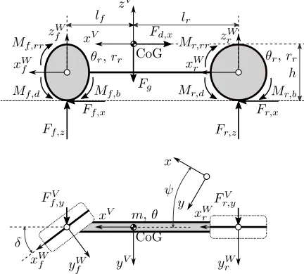
The planar multi-body model (Fig. 1) consists of a chassis with mass m and moment of inertia θ about its vertical axis (zV), and virtual front and rear wheels with moment of inertiaθf,θr about their own rotation axes (yV
f,yVr) representing the complete front and rear axes of the vehicle. The chassis can move longitudinallyxand laterallyy, and rotateψ about its vertical axis. The wheels can rotateρf,ρr about their axes as well. The center of gravity of the vehicle is considered to be constant. The radii of the wheels are noted withrf andrf, the center of gravity height of the vehicle is marked with h, and the horizontal distance between the center of gravity and the front and rear wheel centers are denoted withlf andlf respectively. The inputs of the model are the steering angle of the front wheel δ and the total applied driving Md and braking Mb torques. In the following Subsections 1.3.1 and 1.3.2 superscripts are used to distinguish dynamic quantities in the ground’s (no superscript) vehicle’s (V) and in the wheel’s (W) coordinate system. The coordinate transformations between the different coordinate systems are not detailed due to limited space. Furthermore, all time derivatives are noted with dot (˙).
Fig. 1.Nonlinear single track vehicle model
1.3.1 Dynamics of the Wheels
A dynamic wheel slip model is introduced based on [33] to increase the precision of the simulation in case of near-standstill (drive-off, full braking)
situations, and to enable the usage of explicit ordinary differential equation (ODE) solvers and larger step sizes. The dynamic equations for the front wheel are the following:
¨ ρf=θ1
f
Mf,d−rfFWf,x−Mf,b−Mf,rr
, (5)
˙ sf,x=l1
f,x
rfρ˙f−x˙Wf − |x˙Wf |sf,x
, (6)
˙ sf,y=l1
f,y
−y˙Wf − |x˙Wf |sf,y
. (7)
Eq. (5) represents the motion of the wheel. In case of driving, the total driving torque is distributed by an arbitrary factor ξM between the front Md,f and rear Md,r wheels. In case of braking, ideal break torque distribution (in sense that the longitudinal wheel slip values are equal for the two wheels) is applied to compute the wheel braking torques Mb,f andMb,r. Eqs. (6) and (7) are used to calculate the dynamic longitudinal and lateral wheel slips. The slip dependent longitudinal relaxation length is:
lf,x=max
lf,x,0
1−3DCf,F f,x|sf,x|
,lf,x,min
, (8)
withCf,F =Bf,xCf,xDf, where lf,x,0 and lf,x,min are the longitudinal relaxation lengths at standstill and at wheel spin or lock respectively. Eq. (8) is also valid for the lateral directionlf,yas well, with the substitution of subscriptsxandy. The tire forces are calculated by the Magic Formula:
FfW,x=Dfsin{Cf,xarctan(Bf,xs˜f,x−
E[Bf,xs˜f,x−arctan(Bf,xs˜f,x)])}, (9)
withDf =µfFfW,z, where µf is the static coefficient of friction between tire and road surfaces, and Bf,x, Cf,x, Ef,x are parameters. Eq. (9) is valid for the lateral directionFW
f,y as well, with the substitution of subscriptsxwithy.
To enhance the behavior of the model at very low speeds e.g. when starting from or braking to standstill, a slip damping factor is applied like following:
kf,x= 1 2kf,x,0
1+cosπ|x˙
W f |
vlow
, if ˙xWf ≤vlow
0, if ˙xWf >vlow
, (10)
wherekf,x,0is the damping value zero velocity andvlow is the velocity at which damping is switched off. The
damping is only applied in the longitudinal direction, the damped slip values are:
˜
sf,x=sfx+
kf,x
Cf,F(rfρ˙f−x˙ W
f ), (11)
˜
sf,y=sf,y. (12)
The rolling resistance torque is calculated as follows:
Mf,rr=FfW,zrfsign(rfρ˙f)·
[Arr+Brr|rfρ˙f|+Crr(rfρ˙f)2],
(13)
where Arr, Brr, and Crr are rolling resistance coefficients. Eqs. (5) to (13) are all valid for the rear wheel with changing the subscripts from f tor.
1.3.2 Dynamics of the Chassis
The dynamics of the chassis is now expressed in the inertial coordinate system of the ground. The equations of motion are:
¨ x= 1
m(Ff,x+Fr,x+Fd,x), (14)
¨ y= 1
m(Ff,y+Fr,y+Fd,y), (15)
¨
ψ= 1
θ(lfFVf,y−lrFrV,y). (16) Aerodynamic drag force is applied to the vehicle according to the following:
FV
d,x=12cDAfρAx˙Vx˙V+y˙V, (17) FdV,y=12cDAfρAy˙Vx˙V+y˙V, (18)
wherecD is the drag coefficient andAf is the frontal area of the vehicle, andρAis the mass density of air.
1.3.3 Closed Loop Control
Since the developed motion is described by the temporal course of the vehicle’s state along the trajectory, a mapping is needed between wheel level inputs (steering angle δ, driving Md and brakingMb torque) to some of the state variables to facilitate the usage of input functions meaningful from the perspective of vehicle motion. This mapping is reached by applying closed loop trajectory tracking control. From the view of the optimization problem, arbitrary methods can be used to implement the control. In this paper, two independent linear
quadratic regulator (LQR) controls are used. The longitudinal controller is responsible for the tracking of longitudinal velocity reference vre f as well as the lateral controller follows a yaw-rate ωre f reference. The selection of controllers is of course in close relationship with the input functions applied in the optimization problem, described in Subsection 1.5.
1.4 Constraints
The required end configuration of the vehicle must be formulated in form of constraints for the optimization problem described in Eq. (3). In this work this is happening with application of nonlinear equality constraints. The minimum feasible set of specified end state variables are positionxf,yf and orientation ψf, however it is also reasonable to define the yaw rate ˙ψf. Accordingly, the applied constraint equation is:
C(X) =Xf−X(tf) =
xf yf ψf ˙ ψf
−
x(tf) y(tf) ψ(tf)
˙ ψ(tf)
=0. (19)
1.5 Input Functions
In [17] it is shown that longitudinal velocity and yaw rate can efficiently (relatively small number of parameters enables feasible customization) be parametrized to describe the vehicle’s motion. In current work, longitudinal velocity is always chosen constant (vre f =const.) along the trajectory to reduce the number of free parameters. This choice is not unreasonable because the travel time typically remains in range of a few seconds.
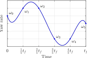
As the yaw-rate input signal, a polynomial
spline profile shown in Fig. 2 is used. The
spline is parametrized by knot points that are placed equidistantly, and by the time span. In current work,
Fig. 2.Yaw-rate reference signal parametrization
a cubic spline is used which means 4 knot point parameters and the travel time parameter additionally. The first knot point is however chosen to be exactly the initial value of yaw-rate of the vehicle ˙ψito avoid jumps in control inputs. Accordingly, the reduced parameter vector is:
pω=ω1 ω2 ω3 tfT. (20)
1.6 Solution of the Planning Problem
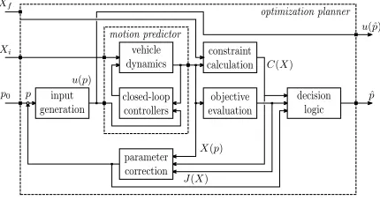
Fig. 3 shows the architecture of how the solution ˆpof the optimization problem represented by Eqs. (1) to (3) is found. The inputs of the optimization process are the current initial state Xi, and the required terminal stateXfof the vehicle, and an initial guess on the input function parameters p0. The initial guess is chosen to the parameters of straight drive, namely:
p0=0 0 0 xf/vre f. (21)
The iteration step begins with the evaluation of the input function (the polynomial spline yaw rate
reference) based on the parameter values. The
response of the controller-vehicle system is then calculated by the following equation:
X(p,t) =Xi+ t
0 f(X(p,τ),u(p,τ)dτ, (22)
which can be solved numerically with the 4th
Runge-Kutta method for instance. Knowing the
trajectory, the objective function (Eq. (4)) and the constraint function (Eq. (19)) are evaluated, and the optimization solver checks if a feasible solution is found. If so, the motion planning is solved. Otherwise, the optimization solver calculates a correction of the parameters based on the objective and constraint values and starts a new iteration step with these corrected values.
Fig. 3.Optimization planner architecture
As an optimization solver, interior point methods, trust region methods or sequential quadratic programming methods can be used.
2 HYBRID APPROACH USING ARTIFICIAL NEURAL NETWORKS
2.1 Basic Concept
The nonlinear optimization based trajectory planning method presented in Section 1 introduces a sophisticated vehicle dynamics-focused approach. This comes at the price of significant computational requirements, which makes the current implementation unable to fulfill real-time applicability. Artificial neural networks have been used for function approximation since a long time. During planning, the optimization planner performs a mapping from the initial and terminal configurations of the vehicle to the appropriate input function parameters that will drive the vehicle accordingly. With the training of an artificial neural network via supervised learning to approximate this mapping, the optimization motion planning algorithm could be substituted. However, the trained neural network will always behave as a black box system. As such, it cannot be applied as a standalone algorithm, because there is no guarantee that it will produce a feasible output in all scenarios. In this paper, two possible applications of an artificial neural network are described, which are operating the network together with the classical model based methods to provide feasible motions with faster computation times.
2.2 Initial Value Generator
The computation time of the optimization planner can be greatly decreased, if the initial guess of the optimized variable p0is already close to the optimal solution. The initial value chosen in Eq. (21) is however obviously not near the optimum. The first idea is to use the neural network to provide a better initial guess instead. As the neural network is trained to provide the optimal solution, its output is expected to be at least close to the optimum considering also the estimation error. The output of the network flows through the whole original optimization loop (Fig. 3, 3rd input), which means that the process will correct a potential infeasible result. In the following, this approach will be referred to asinitialized optimization planner.
2.3 Hybrid Neural Network Planner
state of the vehicle actually reached when driven by the input signals provided by the neural network estimator is compared with the required end state. In case the magnitude of error is not permissible, an emergency trajectory can be used. This solution will be referred to ashybrid nn planner.
Fig. 4.Hybrid NN planner architecture
2.4 Training of Networks
As described in Subsections 2.2 and 2.3, our goal here is to create a network that can substitute the above mentioned trajectory planning algorithm, or at least provide a sufficient initial value guess for the optimizer. Numerous artificial neural networks with different parameter sets were trained to fulfill these tasks.
The network’s input consists of the vehicle’s state variables selected as constraints for the optimization problem in Eq. (19) both at the initial and at the target configurations. Additionally, the initial and final state vectors are both containing the selected constant travel velocity vre f described in Subsection 1.5. The network’s output contains the parameters of the third-order yaw-rate reference spline defined in Eq. (20).
A data set of 16000 lane changing and curved lane keeping trajectory samples for training was generated with the model-based optimization proposed in Section 1. From the start configuration of:
Xi=xi yi ψi ψ˙i viT
=0 0 0 0 vre fT,
(23)
the target state vectors are defined by the following equations and ranges:
Xf =
xf yf ψf ˙ ψf
vf
=
50. . .100 m −0.15xf. . .0.15xf m −0.1ψC. . .1.2ψC rad
vre fsin(xψf f) rad/s vre f m/s
, (24)
whereψC=2arctan(yxff)is the yaw angle of circular path, andvre f is chosen to 20 m/s. The ranges were determined by vehicle simulations to cover the whole dynamically feasible region ahead of the vehicle, and the edges are selected to reach even extreme dynamical parameters (e.g. lateral acceleration up to near 1g). A portion of the generated sample trajectories is shown in Fig. 5. In Section 3, all the figures will show the results regarding to these trajectories, in the ascending order of maximal lateral acceleration.
Fig. 5.Sample trajectories
The core of the complex problem of computing dynamically feasible motions is irrelevant from the perspective of the training of an artificial
neural network. The problem that the network
is needed to provide a solution for is handled
as a general function approximation. In order
to explore the benefits of different networks to reach the best regression possible, several parameters defining the training or the network itself were
used in every possible combinations. Although
Levenberg-Marquandt algorithm is well-known for its superior performance in function approximation, in order to perform a more comprehensive study on the training process, Broyden–Fletcher–Goldfarb–Shanno (BFGS) and resilient back-propagation algorithms were also targets of examination.
Regarding network architecture two variants defining the connection of the adjacent layers differently were tested: feed-forward and cascade structures.
The input layer defined by the input vectors consists of 10 neurons, while the output layer using linear transfer function is of 4 neuron size, corresponding to the output vector defining the planned yaw-rate reference. Hidden layers use tangent sigmoid transfer function were examined in seven different structures: one layer sized [10] and [20], two layers sized [10; 8], [20; 8], [30; 10], three layers sized [10; 20; 8], [20; 10; 8]. The decomposition of the training data set for train, validation and test sets is also a factor worth consideration regarding the result of the training. Five different ratios were tested: [80:10:10], [70:15:15], [60:25:15], [60:15:25] and [50:25:25]. Every network with different parameter sets were trained five times with different initial values and were saved with the weights and biases culminating in the best test results, in order to exclude the effect of the potentially occurring error of finding local extremes instead of the global minimum of the error function during the training process. As it was expected, the training algorithm resulting in the fastest convergence was the Levenberg-Marquandt method, which resulted the networks to reach the performance goal in an order of magnitude faster than the networks trained with either BFGS or resilient back-propagation algorithm. Based on the test results, one hidden layer sized cascade networks and networks with multiple hidden layers provided the best performance on the test data set, while no major difference was occurring regarding the number of neurons.
In respect to regression, the trained networks perform the function approximation task with mean squared error values around 10-2on the test data set.
3 TESTING AND BENCHMARKING
3.1 Comparison of Run-time
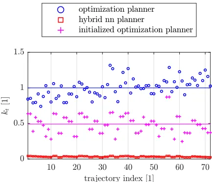
Fig. 6 shows the run-time of the motion planning algorithms normalized to the run-time of the optimization planner:
kt(i) =t j calc(i)
tcalcopt(i), (25)
where i is the index of the trajectory, tcalcopt(i) is the calculation time of the ith trajectory with the optimization planner, and tcalcj (i) is the calculation time with planner j. The average planning time of the initialized optimization planner is decreased
significantly by 51 %. The speed-up is even more essential in case of thehybrid nn planner, the average planning time is here decreased by 96.63 %.
Fig. 6.Normalized run-times
As the run-time of the optimization planner is in the magnitude of 1 s, the results show, that even the current MATLAB based implementation of thehybrid nn planner may be suitable for real-time application from the perspective of planning time.
3.2 Comparison of Performance
3.2.1 Performance of Reference Parameter Estimation The deviation between the planned reference parameters normalized to the output parameters of the optimization planner shown in Fig. 7 is calculated by:
kp(i) = p
j(i)−popt(i) popt(i)
, (26)
wherepopt(i)is the parameter vector generated by the optimization plannerin case of theithtrajectory, and pj(i)is the parameter vector in case of planner j.
Fig. 7.Normalized deviation of reference parameters
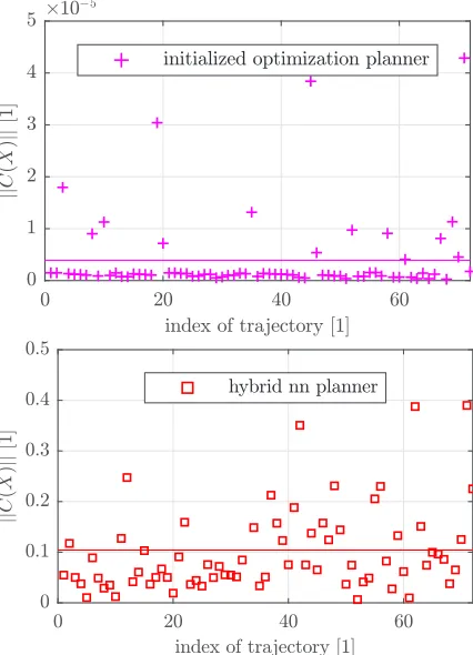
3.2.2 Deviations in Vehicle State
The final value of state constraints, namely the euclidean norm of deviation between prescribed Xf
and actually reached X(tf) end states of the vehicle
is shown in Fig. 8. The deviation of the initialized
optimization planner is again negligible, as the
constraint tolerance of the nonlinear optimization solver is set to a sufficiently low value (10-4). In case
of thehybrid nn planner, the norm of state constraint is noticeable. This is expected based on the results in Fig. 7. The main contributor to the total value is the deviation in the final vehicle position, so we can declare a maximal position error of approximately 40 cm after the whole planned motion (≈2 s), which is remarkable.
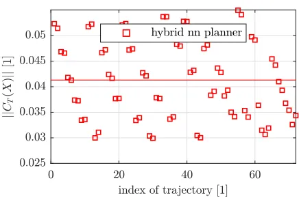
However, the motions planned by the algorithm are actually only meant to be executed until the result of the next trajectory planning cycle is being calculated (≈50 ms), and new trajectories are expected to be planned as frequently as possible. The vehicle state deviation when considering only the executed part of the trajectory is calculated as follows:
CT(X) =Xopt(tcalcnn )−Xnn(tcalcnn ), (27)
Fig. 8.Final deviation of vehicle state
where Xopt(·)and Xnn(·) are the state of the vehicle
in case of the optimization planner and the hybrid
nn planner respectively, and tnn
calc is the maximal
calculation time with thehybrid nn planner.
Fig. 9.Final deviation of vehicle state considering only the driven part
The results in Fig. 9 show that the state deviations are in a feasible range (with a maximal position deviation of approximately 1.3 mm) when considering only the driven part of the motion.
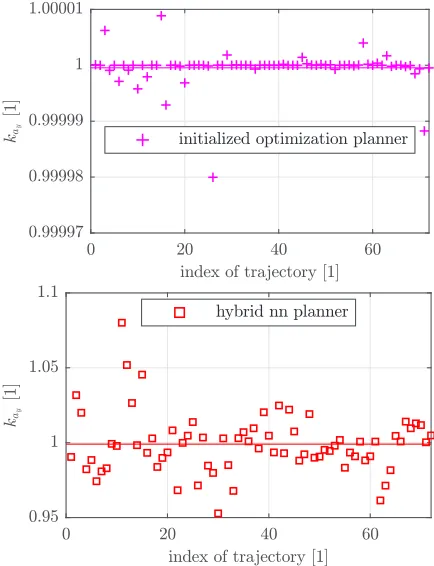
3.2.3 Influences on the Optimality Criteria
As the proposed optimization planner provides an optimal motion with respect to the comfort of the passengers with the minimization of lateral acceleration ¨yV, a corresponding comparison is also
advisable and is shown in Fig. 10. The maximal value of lateral acceleration normalized to the maximal lateral acceleration developing in case of the
optimization planner is calculated by the following
equation:
kay=
max(y¨V,j(i))
max(y¨V,opt(i)), (28)
where ¨yV,opt(i) is the lateral acceleration of the ith
trajectory in case of the optimization planner, and ¨
yV,j(i)is the lateral acceleration in case of planner j.
Fig. 10.Normalized maximal lateral accelerations
Once again, the performance of the initialized optimization planneris virtually the same, as expected.
The hybrid nn planner produces a maximal increase
of approximately 7.85 %, while the average stays around zero deviation. The value of maximal lateral acceleration is even smaller in several cases, which is possible by the violation of the prescribed end configuration.
3.3 Validation of Benchmark Results
As the run-time of the hybrid nn planner enables real-time application, the benchmark results for this algorithm were validated with the industrial vehicle simulation software IPG CarMaker to prepare the application on a test car. The examination with a highly accurate, close-to-real environment was important, bacause the benchmark results in Section 3.2 were evaluated using the same single-track vehicle model that is employed in the optimization planner, which means that the deviations between the nominal system and a real vehicle due to unmodeled dynamics and changing environment conditions are not considered there.
Fig. 11.Lane change maneuver in CarMaker
Fig. 11 shows a lane change maneuver performed by the proposed planner in the CarMaker environment. The virtual test vehicle is chosen as a mid-size passenger car. The main parameters of the chassis (m, θ, lf, lr) and the wheels (rf, rr, µf, µr) of the
vehicle motion estimator module of the planner were not adjusted exactly to the simulated vehicle to model the inevitable differences between the nominal and the actual systems (e.g. mass depending on the number of passengers).
The CarMaker simulation results on Fig. 12 show that the deviations of the vehicle’s final state from the planning target are higher than the ones on Fig. 8 but remain in case of almost every trajectory under a position error of 1 m. The deviation after the time frame necessary for the planning of the following trajectory is typically in a range of a few centimeters as shown in Fig. 13, which is not very small but is still in a feasible range considering that a suitable safety margin is used for collision avoidance.
In terms of the highest lateral acceleration along the planned motion, Fig. 14 even shows an
Fig. 12.Final deviation of vehicle state in CarMaker
Fig. 13.Final deviation of vehicle state considering only the driven part in CarMaker
improvement in average. Of course, this is mainly possible due to the violation of the state constraints, but the overall performance is very similar to the one on Fig. 10.
4 CONCLUSIONS AND OUTLOOK
In this paper a nonlinear optimization based trajectory planning algorithm is proposed to generate dynamically feasible, comfortable, and configurable motion for highly automated or autonomous road vehicles with the model-based prediction of the vehicle’s motion. The main drawback of the developed approach is the significant computation time, which jeopardizes real-time usage even with a possible move from the current MATLAB based implementation to a faster one, e.g. in C++.
To overcome this issue, two hybrid approaches are suggested with the application of an artificial neural network. Based on a dataset generated off-line with the optimization planner, the network is trained to solve the motion planning problem by the approximation
Fig. 14.Normalized maximal lateral accelerations in CarMaker
of the optimization planner’s behavior. The first method uses the output of the neural network as an initial guess of the optimization process. This halves the run-time of the planning while maintaining the same performance regarding dynamical feasibility and motion optimality. The second algorithm skips the optimization entirely, using the neural network’s output directly. The trajectory of the vehicle is calculated with the motion predictor applied in the optimization planner. The plausibility of the network’s output is checked by the comparison of the prescribed and actually reached final states, which eliminates the problematic of the neural network being a black-box system. Although there are remarkable differences between the motions planned by the neural network and the optimization process when considering the whole trajectory, the deviations are in a feasible range if only the part of the motion which is meant to be actually driven is dealt with. The significantly decreased computation time can even enable the real-time usage of the proposed hybrid approach.
network, an even more accurate twin-track vehicle model could be used to evaluate the trajectories. As the authors are developing the optimization planner to include obstacle avoidance internally in the optimization problem, a corresponding extension of the presented neural network approach would also be an interesting opportunity.
5 ACKNOWLEDGEMENTS
The research reported in this paper was supported by the Higher Education Excellence Program of the Ministry of Human Capacities in the frame of Artificial Intelligence research area of Budapest University of Technology and Economics (BME FIKPMI/FM).
EFOP-3.6.3-VEKOP-16-2017-00001: Talent
management in autonomous vehicle control
technologies- The Project is supported by the Hungarian Government and co-financed by the European Social Fund.
6 REFERENCES
[1] European Comission Mobility and Transport DG, Brussels, (2016),Road Safety in the European Union. https://ec.europa.eu/transport/road_safety/home_en. [2] A. C. Mersky, C. Samaras, (2016), “Fuel economy
testing of autonomous vehicles,” Transportation Research Part C: Emerging Technologies, vol. 65, pp. 31 – 48.
[3] Y. Chen, J. Gonder, S. Young„ E. Wood, (2017), “Quantifying autonomous vehicles national fuel consumption impacts: A data-rich approach,” Transportation Research Part A: Policy and Practice. [4] T. Tettamanti, I. Varga„ Z. Szalay, (2016), “Impacts
of autonomous cars from a traffic engineering perspective,” Periodica Polytechnica Transportation Engineering, vol. 44, no. 4, pp. 244–250.
[5] B. Paden, M. Cap, S. Z. Yong, D. Yershov„ E. Frazzoli, (2016), “A survey of motion planning and control techniques for self-driving urban vehicles,” IEEE Transactions on Intelligent Vehicles, vol. 1, pp. 33–55. [6] H. Vorobieva, N. Minoiu-Enache, S. Glaser„
S. Mammar, (2013), “Geometric continuous-curvature path planning for automatic parallel parking,” in2013 10th IEEE International Conference on Networking, Sensing and Control (ICNSC), pp. 418–423.
[7] M. Boryga, (2014), “Trajectory planning of end-effector for path with loop,” Strojniški vestnik - Journal of Mechanical Engineering, vol. 60, no. 12, pp. 804–814. [8] V. T. Minh, J. Pumwa, (2014), “Feasible path planning
for autonomous vehicles,” Mathematical Problems in Engineering, vol. 2014.
[9] X. Li, Z. Sun, Z. He, Q. Zhu„ D. Liu, (2015), “A practical trajectory planning framework for autonomous ground vehicles driving in urban environments,” in2015 IEEE Intelligent Vehicles Symposium (IV), pp. 1160–1166.
[10] E. W. Dijkstra, (1959), “A note on two problems in connexion with graphs,” Numer. Math., vol. 1, pp. 269–271.
[11] S. Liu, K. Mohta, N. Atanasov„ V. Kumar, (2018), “Search-based motion planning for aggressive flight in se(3),”IEEE Robotics and Automation Letters, vol. 3, pp. 2439–2446.
[12] M. Likhachev, D. Ferguson, G. J. Gordon, A. Stentz„ S. Thrun, (2005), “Anytime dynamic a*: An anytime, replanning algorithm.,” inICAPS, pp. 262–271. [13] M. Montemerlo, J. Becker, S. Bhat, et al., (2008),
“Junior: The stanford entry in the urban challenge,” Journal of field Robotics, vol. 25, no. 9, pp. 569–597. [14] K. R. Jayasree, P. R. Jayasree„ A. Vivek, (2017),
“Smoothed rrt techniques for trajectory planning,”
in 2017 International Conference on Technological
Advancements in Power and Energy ( TAP Energy), pp. 1–8.
[15] L. E. Dubins, (1957), “On curves of minimal length with a constraint on average curvature, and with prescribed initial and terminal positions and tangents,” American Journal of Mathematics, vol. 79, no. 3, pp. 497–516. [16] O. Arslan, K. Berntorp„ P. Tsiotras, (2017),
“Sampling-based algorithms for optimal motion planning using closed-loop prediction,” in 2017 IEEE International Conference on Robotics and Automation (ICRA), pp. 4991–4996.
[17] T. M. Howard, A. Kelly, (2007), “Optimal rough terrain trajectory generation for wheeled mobile robots,”The International Journal of Robotics Research, vol. 26, no. 2, pp. 141–166.
[18] D. Ferguson, T. M. Howard„ M. Likhachev, (2008), “Motion planning in urban environments: Part i,” in 2008 IEEE/RSJ International Conference on Intelligent Robots and Systems, pp. 1063–1069.
[19] B. Li, Z. Shao, (2015), “A unified motion planning method for parking an autonomous vehicle in the presence of irregularly placed obstacles,” Knowledge-Based Systems, vol. 86, pp. 11 – 20. [20] S. X. Yang, M. Meng, (2001), “Neural network
approaches to dynamic collision-free trajectory generation,” IEEE Transactions on Systems, Man, and Cybernetics, Part B (Cybernetics), vol. 31, pp. 302–318.
[21] L. Liu, J. Hu, Y. Wang„ Z. Xie, (2017), “Neural network-based high-accuracy motion control of a class of torque-controlled motor servo systems with input saturation,” Strojniški vestnik - Journal of Mechanical Engineering, vol. 63, no. 9, pp. 519–528.
[22] I. Engedy, G. Horvath, (2009), “Artificial neural network based mobile robot navigation,” in 2009 IEEE International Symposium on Intelligent Signal Processing, pp. 241–246.
[23] H. Qu, S. X. Yang, A. R. Willms„ Z. Yi, (2009), “Real-time robot path planning based on a modified pulse-coupled neural network model,” IEEE Transactions on Neural Networks, vol. 20, pp. 1724–1739.
[24] D. Janglová, (2004), “Neural networks in mobile robot motion,” International Journal of Advanced Robotic Systems, vol. 1, no. 1, p. 2.
12 Ferenc Hegedüs, Tamás Bécsi, Szilárd Aradi, Péter Gáspár
[1] European Commission Mobility and Transport (2016). Road Safety in the European Union, from https://ec.europa.eu/ transport/road_safety/home_en, accessed on 2018-10-18. [2] Mersky, A.C., Samaras, C. (2016). Fuel economy testing
of autonomous vehicles. Transportation Research Part C: Emerging Technologies, vol. 65, p. 31-48, DOI:10.1016/j. trc.2016.01.001.
[3] Chen, Y., Gonder, J., Young, S., Wood, E. (2017). Quantifying autonomous vehicles national fuel consumption impacts: A data-rich approach. Transportation Research Part A: Policy and Practice, in press, DOI:10.1016/j.tra.2017.10.012. [4] Tettamanti, T., Varga, I., Szalay, Z. (2016). Impacts of
autonomous cars from a traffic engineering perspective.
Periodica Polytechnica Transportation Engineering, vol. 44, no. 4, p. 244-250, DOI:10.3311/PPtr.9464.
[5] Paden, B., Čap, M., Yong, S.Z., Yershov, D., Frazzoli, E.
(2016). A survey of motion planning and control techniques for self-driving urban vehicles. IEEE Transactions on Intelligent Vehicles, vol. 1, no. 1, p. 33-55, DOI:10.1109/ TIV.2016.2578706.
[6] Vorobieva, H., Minoiu-Enache, N., Glaser, S., Mammar, S., Mammar, S. (2013). Geometric continuous-curvature path planning for automatic parallel parking. 10th IEEE International
Conference on Networking, Sensing and Control, p. 418-423, DOI:10.1109/ICNSC.2013.6548775.
[7] Boryga, M. (2014). Trajectory planning of end-effector for path with loop. Strojniški vestnik - Journal of Mechanical Engineering, vol. 60, no. 12, p. 804-814, DOI:10.5545/sv-jme.2014.1965.
[8] Minh, V.T., Pumwa, J. (2014). Feasible path planning for autonomous vehicles. Mathematical Problems in Engineering,
vol. 2014, art. ID 317494, DOI:10.1155/2014/317494.
[9] Li, X., Sun, Z., He, Z., Zhu, Q., Liu, D. (2015). A practical
trajectory planning framework for autonomous ground vehicles driving in urban environments. IEEE Intelligent Vehicles Symposium (IV), p. 1160-1166, DOI:10.1109/ IVS.2015.7225840.
[10] Dijkstra, E.W. (1959). A note on two problems in connexion
with graphs. Numerische Mathematik, vol. 1, no. 1, p. 269-271, DOI:10.1007/BF01386390.
[11] Liu, S., Mohta, K., Atanasov, N., Kumar, V. (2018). Search-based motion planning for aggressive flight in SE(3). IEEE Robotics and Automation Letters, vol. 3, no. 3, p. 2439-2446, DOI:10.1109/LRA.2018.2795654.
[12] Likhachev, M., Ferguson, D., Gordon, G., Stentz, A., Thrun,
S. (2005). Anytime dynamic A*: An anytime, replanning algorithm, The International Conference on Automated Planning and Scheduling, p. 262-271.
[13] Montemerlo, M., Becker, J., Bhat, S., et al. (2008). Junior: The Stanford entry in the urban challenge. Journal of Field Robotics, vol. 25, no. 9, p. 569-597, DOI:10.1002/rob.20258. [14] Jayasree, K.R., Jayasree, P.R., Vivek, A. (2017). Smoothed RRT
techniques for trajectory planning. International Conference on Technological Advancements in Power and Energy, p. 1-8, DOI:10.1109/TAPENERGY.2017.8397376.
[15] Dubins, L.E. (1957). On curves of minimal length with
a constraint on average curvature, and with prescribed initial and terminal positions and tangents. American Journal of Mathematics, vol. 79, no. 3, p. 497-516, DOI:10.2307/2372560.
[16] Arslan, O., Berntorp, K., Tsiotras, P. (2017). Sampling-based
algorithms for optimal motion planning using closed-loop prediction. IEEE International Conference on Robotics and Automation, p. 4991-4996, DOI:10.1109/ICRA.2017.7989581. [17] Howard, T. M., Kelly, A. (2007). Optimal rough terrain trajectory
generation for wheeled mobile robots. The International Journal of Robotics Research, vol. 26, no. 2, p. 141-166,
DOI:10.1177/0278364906075328.
[18] Ferguson, D., Howard, T. M. Likhachev, M. (2008). Motion
planning in urban environments: Part I. IEEE/RSJ International Conference on Intelligent Robots and Systems, p. 1063-1069, DOI:10.1109/IROS.2008.4651120.
[19] Li, B., Shao, Z. (2015). A unified motion planning method for parking an autonomous vehicle in the presence of irregularly placed obstacles. Knowledge-Based Systems, vol. 86, p. 11-20, DOI:10.1016/j.knosys.2015.04.016.
[20] Yang, S.X., Meng, M. (2001). Neural network approaches to dynamic collision-free trajectory generation. IEEE Transactions on Systems, Man, and Cybernetics, Part B (Cybernetics), vol. 31, no. 3, p. 302-318, DOI:10.1109/3477.931512.
[21] Liu, L., Hu, J., Wang, Y. Xie, Z. (2017). Neural network-based high-accuracy motion control of a class of torque-controlled motor servo systems with input saturation. Strojniški vestnik - Journal of Mechanical Engineering, vol. 63, no. 9, p. 519-528, DOI:10.5545/sv-jme.2016.4282.
[23] Qu, H., Yang, S.X., Willms, A.R., Yi, Z. (2009). Real-time robot path planning based on a modified pulse-coupled neural network model. IEEE Transactions on Neural Networks, vol. 20, no. 11, p. 1724-1739, DOI:10.1109/TNN.2009.2029858. [24] Janglová, D. (2004). Neural networks in mobile robot motion.
International Journal of Advanced Robotic Systems, vol. 1, no. 1, p. 15-22, DOI:10.5772/5615.
[25] Tai, L., Paolo, G., Liu, M. (2017). Virtual-to-real deep reinforcement learning: Continuous control of mobile robots for mapless navigation. IEEE/RSJ International Conference on Intelligent Robots and Systems, p. 31-36, DOI:10.1109/ IROS.2017.8202134.
[26] Plessen, M.G. (2017). Automating vehicles by deep
reinforcement learning using task separation with hill climbing. CoRR, vol. abs/1711.10785.
[27] Velagic, J., Osmic, N., Lacevic, B. (2008). Neural network
controller for mobile robot motion control. International Journal of Electrical and Computer Engineering, vol. 2, no. 11, p. 2471-2476.
[28] Gorinevsky, D., Kapitanovsky, A., Goldenberg, A. (1996). Neural
network architecture for trajectory generation and control of automated car parking. IEEE Transactions on Control Systems Technology, vol. 4, no. 1, p. 50-56, DOI:10.1109/87.481766.
[29] Yim, Y., Oh, S.-Y. (2004). Modeling of vehicle dynamics from
real vehicle measurements using a neural network with two-stage hybrid learning for accurate long-term prediction. IEEE Transactions on Vehicular Technology, vol. 53, no. 4, p. 1076-1084, DOI:10.1109/TVT.2004.830145.
[30] Bellem, H., Schönenberg, T., Krems, J.F., Schrauf, M. (2016).
Objective metrics of comfort: Developing a driving style
for highly automated vehicles. Transportation Research Part F: Traffic Psychology and Behaviour, vol. 41, p. 45-54, DOI:10.1016/j.trf.2016.05.005.
[31] Hegedüs, F., Bécsi, T., Aradi, S. (2017). Dynamically feasible
trajectory planning for road vehicles in terms of sensitivity and robustness. Transportation Research Procedia, vol. 27, p. 799-807, DOI:10.1016/j.trpro.2017.12.110.
[32] Hegedüs, F., Bécsi, T., Aradi, S., Gápár, P. (2017). Model based trajectory planning for highly automated road vehicles. IFAC-PapersOnLine, vol. 50, no. 1, p. 6958-6964, DOI:10.1016/j. ifacol.2017.08.1336.
[33] Pacejka, H.B. (2012). Chapter 8 - Applications of transient tire models. Pacejka, H.B. (ed.) Tire and Vehicle Dynamics (3rd ed.)