Coherence Functions with Applications in Large-Margin Classification Methods

(1)

Coherence Functions with Applications

in Large-Margin Classification Methods

Zhihua Zhang [email protected]

Dehua Liu [email protected]

Guang Dai [email protected]

College of Computer Science and Technology Zhejiang University

Hangzhou, Zhejiang 310027, China

Michael I. Jordan [email protected]

Computer Science Division and Department of Statistics University of California

Berkeley, CA 94720-1776, USA

Editor:Xiaotong Shen

Abstract

Support vector machines (SVMs) naturally embody sparseness due to their use of hinge loss func-tions. However, SVMs can not directly estimate conditional class probabilities. In this paper we propose and study a family ofcoherence functions, which are convex and differentiable, as sur-rogates of the hinge function. The coherence function is derived by using the maximum-entropy principle and is characterized by a temperature parameter. It bridges the hinge function and the logit function in logistic regression. The limit of the coherence function at zero temperature corresponds to the hinge function, and the limit of the minimizer of its expected error is the minimizer of the expected error of the hinge loss. We refer to the use of the coherence function in large-margin clas-sification as “C-learning,” and we present efficient coordinate descent algorithms for the training of regularizedC-learning models.

Keywords: large-margin classifiers, hinge functions, logistic functions, coherence functions,C -learning

1. Introduction

Large-margin classification methods have become increasingly popular since the advent of boost-ing (Freund, 1995), support vector machines (SVM) (Vapnik, 1998) and their variants such asψ -learning (Shen et al., 2003). Large-margin classification methods are typically devised based on a majorization-minimization procedure, which approximately solves an otherwise intractable opti-mization problem defined with the 0-1 loss. For example, the conventional SVM employs a hinge loss, the AdaBoost algorithm employs the exponential loss, and ψ-learning employs a so-called

ψ-loss, as majorizations of the 0-1 loss.

(2)

Recent developments in the former vein focus on the use of theℓ1penalty (Tibshirani, 1996) or the elastic-net penalty (a mixture of theℓ1andℓ2 penalties) (Zou and Hastie, 2005) instead of theℓ2 penalty which is typically used in large-margin classification methods. As for non-differentiable losses, the paradigm case is the hinge loss function that is used for the SVM and which leads to a sparse expansion of the discriminant function.

Unfortunately, the conventional SVM does not directly estimate a conditional class probability. Thus, the conventional SVM is unable to provide estimates of uncertainty in its predictions—an important desideratum in real-world applications. Moreover, the non-differentiability of the hinge loss also makes it difficult to extend the conventional SVM to multi-class classification problems. Thus, one seemingly natural approach to constructing a classifier for the binary and multi-class problems is to consider a smooth loss function, while an appropriate penalty is employed to maintain the sparseness of the classifier. For example, regularized logistic regression models based on logit losses (Friedman et al., 2010) are competitive with SVMs.

Of crucial concern are the statistical properties (Lin, 2002; Bartlett et al., 2006; Zhang, 2004) of the majorization function for the original 0-1 loss function. In particular, we analyze the statistical properties of extant majorization functions, which are built on the exponential, logit and hinge func-tions. This analysis inspires us to propose a new majorization function, which we call acoherence functiondue to a connection with statistical mechanics. We also define a loss function that we refer to as

C

-loss based on the coherence function.

The

C

-loss is smooth and convex, and it satisfies a Fisher-consistency condition—a desirable statistical property (Bartlett et al., 2006; Zhang, 2004). The

C

-loss has the advantage over the hinge loss that it provides an estimate of the conditional class probability, and over the logit loss that one limiting version of it is just the hinge loss. Thus, the

C

-loss as well as the coherence function have several desirable properties in the context of large-margin classifiers.

In this paper we show how the coherence function can be used to develop an effective approach to estimating the class probability of the conventional binary SVM. Platt (1999) first exploited a sigmoid link function to map the SVM outputs into probabilities, while Sollich (2002) used loga-rithmic scoring rules (Bernardo and Smith, 1994) to transform the hinge loss into the negative of a conditional log-likelihood (i.e., a predictive class probability). Recently, Wang et al. (2008) devel-oped an interval estimation method. Theoretically, Steinwart (2003) and Bartlett and Tewari (2007) showed that the class probability can be asymptotically estimated by replacing the hinge loss with a differentiable loss. Our approach also appeals to asymptotics to derive a method for estimating the class probability of the conventional binary SVM.

Using the

C

-loss, we devise new large-margin classifiers which we refer to as

C

-learning. To maintain sparseness, we use the elastic-net penalty in addition to

C

-learning. We in particular propose two versions. The first version is based on reproducing kernel Hilbert spaces (RKHSs) and it can automatically select the number of support vectors via penalization. The second version focuses on the selection of features again via penalization. The classifiers are trained by coordinate descent algorithms developed by Friedman et al. (2010) for generalized linear models.

(3)

2. Large-Margin Classifiers

We consider abinaryclassification problem with a set of training data

T

=_{xi,yi}n₁, where xi∈

X

_⊂_Rd_{is an input vector and}_y

i∈

Y

={1,−1}is the corresponding class label. Our goal is to find

a decision function f(x)over a measurable function class

F

. Once such an f(x)is obtained, the classification rule isy=sign(f(x))where sign(a) =1,0,₋1 according toa>0, a=0 ora<0. Thus, we have thatxis misclassified if and only ify f(x)_≤0 (here we ignore the case that f(x) =0). Letη(x) =Pr(Y =1_|X =x) be the conditional probability of class 1 givenx and letP(X,Y)

be the probability distribution over

X

_×

Y

. For a measurable decision function f(x):

X

_→_R, the expected error atxis then defined by

Ψ(f(x)) =E(I_[_{Y f}₍_X₎_≤₀_]_|X=x) =I_[_f₍x)≤0]η(x) +I[f(x)>0](1−η(x)),

whereI_[_#_]=1 if # is true and 0 otherwise. The generalization error is

Ψf =EPI[Y f(X)≤0]=EX

I[f(X)≤0]η(X) +I[f(X)>0](1−η(X))

,

where the expectationEP is taken with respect to the distributionP(X,Y)andEX denotes the

ex-pectation over the input data

X

. The optimal Bayes error is ˆΨ=EPI[Y(2η(X)−1)≤0], which is the

minimum ofΨf with respect to measurable functions f.

A classifier is a classification algorithm which finds a measurable function fT :

X

→Rbased on the training data

T

. We assume that the(xi,yi)in

T

are independent and identically distributed

fromP(X,Y). A classifier is said to beuniversally consistentif

lim

n_→∞ΨfT =

ˆ

Ψ

holds in probability for any distribution P on

X

_×

Y

. It is strongly universally consistent if the condition limn→∞ΨfT =Ψˆ is satisfied almost surely (Steinwart, 2005).

The empirical generalization error on the training data

T

is given by

Ψemp=

1

n

∑

i=1

I_[_y_i_f₍xi)≤0].

Given that the empirical generalization error Ψemp is equal to its minimum value zero when all

training data are correctly classified, we wish to use Ψemp as a basis for devising classification

algorithms. However, the corresponding minimization problem is computationally intractable.

2.1 Surrogate Losses

A wide variety of classifiers can be understood as minimizers of a continuoussurrogate lossfunction

φ(y f(x)), which upper bounds the 0-1 lossI_[_{y f}₍_x₎_≤₀_]. Corresponding toΨ(f(x))andΨf, we denote

R(f(x)) =φ(f(x))η(x) +φ(₋f(x))(1₋η(x))and

Rf =EP[φ(Y f(X))] =EX

φ(f(X))η(X) +φ(₋f(X))(1₋η(X)) .

For convenience, we assume thatη_∈[0,1]and define the notation

(4)

Exponential Loss Logit Loss Hinge Loss Squared Hinge Loss

exp[₋y f(x)/2] log[1+exp(₋y f(x))] [1₋y f(x)]+ ([1−y f(x)]+)2

Table 1: Surrogate losses for margin-based classifier.

The surrogate φ is said to be Fisher consistent, if for every η_∈[0,1] the minimizer of R(η,f)

with respect to f exists and is unique and the minimizer (denoted ˆf(η)) satisfies sign(fˆ(η)) =

sign(η₋1/2) (Lin, 2002; Bartlett et al., 2006; Zhang, 2004). Since sign(u) =0 is equivalent to

u=0, we have that ˆf(1/2) =0. Substituting ˆf(η) into R(η,f), we also define the following notation:

ˆ

R(η) =inf

f R(η,f) =R(η,

ˆ

f(η)).

The difference betweenR(η,f)and ˆR(η)is

△R(η,f) =R(η,f)₋R(η) =ˆ R(η,f)₋R(η,fˆ(η)).

When regarding f(x) andη(x) as functions of x, it is clear that ˆf(η(x))is the minimizer of

R(f(x))among all measurable function class

F

. That is, ˆ

f(η(x)) =argmin

f(x)∈F

R(f(x)).

In this setting, the difference betweenRf andEX[R(fˆ(η(X)))](denotedRfˆ) is given by △Rf =Rf−R_fˆ=EX△R(η(X),f(X)).

If ˆf(η) is invertible, then the inverse function ˆf−1(f(x))over

F

can be regarded as a class-conditional probability estimate given thatη(x) = fˆ−1(fˆ(x)). Moreover, Zhang (2004) showed that △Rf is the expected distance between the conditional probability ˆf−1(f(x))and the true conditional

probabilityη(x). Thus, minimizingRf is equivalent to minimizing the expected distance between

ˆ

f−1(f(x))andη(x).

Table 1 lists four common surrogate functions used in large-margin classifiers. Here [u]+=

max_{u,0_} is a so-called hinge function and ([u]+)2= (max{u,0})2 is a squared hinge function

which is used for developing the ℓ2-SVM (Cristianini and Shawe-Taylor, 2000). Note that we typically scale the logit loss to equal 1 at y f(x) =0. These functions are convex and the upper bounds of I_[_{y f}₍_x₎_≤₀_]. Moreover, they are Fisher consistent. In particular, the following result has been established by Friedman et al. (2000) and Lin (2002).

Proposition 1 Assume that 0 < η(x) < 1 and η(x) ₆= 1/2. Then, the minimizers of E(exp[₋Y f(X)/2]_|X =x) andE(log[1+exp(₋Y f(X))]_|X =x) are both fˆ(x) =log₁₋η(_ηx₍)_x₎, the minimizer of E [1₋Y f(X)]+|X =x is fˆ(x) =sign(η(x)−1/2), and the minimizer of E ([1− Y f(X)]+)2|X=xis fˆ(x) =2η(x)−1.

When the exponential or logit loss function is used, ˆf−1(f(x)) exists. It is clear thatη(x) =

ˆ

f−1(fˆ(x)). For any f(x)_∈

F

, we denote the inverse function by ˜η(x), which is ˜

η(x) =fˆ−1(f(x)) = 1

1+exp(₋f(x)).

(5)

2.2 The Regularization Approach

Given a surrogate loss functionφ, a large-margin classifier typically solves the following optimiza-tion problem:

min

f_∈F 1

n

∑

i=1

φ(yif(xi)) +γJ(h),

where f(x) =α+h(x), J(h) is a regularization term to penalize model complexity and γis the degree of penalization.

Suppose that f =α+h∈(_{1_}+

H

_K)where

H

_K is a reproducing kernel Hilbert space (RKHS) (Wahba, 1990) induced by a reproducing kernelK(_·,_·):

X

_×

X

_→_R. Findingf(x)is then formulated as a regularization problem of the form

min

f∈HK

( 1

n

∑

i=1

φ(yif(xi)) +

γ

2khk 2 HK

)

, (1)

where_khk2

HK is the RKHS norm. By the representer theorem, the solution of (1) is of the form

f(xi) =α+ n

∑

j=1

βjK(xi,xj) =α+k′iβ, (2)

where β = (β1, . . . ,βn)′ and ki = (K(xi,x1), . . . ,K(xi,xn))′. Noticing that

kh_k2_H

K=∑

n

i,j=1K(xi,xj)βiβjand substituting (2) into (1), we obtain the minimization problem with

respect toαandβas

min

α,β

1

n

∑

i=1

φ(yi(α+k′iβ)) +

γ

2β

′_K_β_,

whereK= [k1, . . . ,kn]is then×n kernel matrix. SinceKis symmetric and positive semidefinite,

the termβ′Kβis in fact an empirical RKHS norm on the training data.

In particular, the conventional SVM defines the surrogateφ(_·)as the hinge loss and solves the following optimization problem:

min

f∈F 1

n

∑

i=1

[1₋yi(α+k′iβ)]++

γ

2β

′_K_β_. ₍₃₎

In this paper, we are especially interested inuniversal kernels, namely, kernels whose induced RKHS is dense in the space of continuous functions over

X

(Steinwart, 2001). The Gaussian RBF kernel is such an example.

2.3 Methods for Class Probability Estimation of SVMs

Let ˆf(x)be the solution of the SVM problem in (3). In an attempt to address the problem of class probability estimation for SVMs, Sollich (2002) proposed a class probability estimate

ˆ

η(x) =

( ₁

1+exp(−2 ˆf(x)) if|fˆ(x)| ≤1,

1

1+exp[−(fˆ(x)+sign(fˆ(x)))] otherwise.

(6)

Another proposal for obtaining class probabilities from SVM outputs was developed by Platt (1999), who employed a post-processing procedure based on the parametric formula

ˆ

η(x) = 1

1+exp(Afˆ(x) +B),

where the parameters AandB are estimated via the minimization of the empirical cross-entropy error over the training data set.

Wang et al. (2008) proposed a nonparametric form obtained from training a sequence of weighted classifiers:

min

f_∈F 1

n

(1₋πj)

∑

yi=1

[1₋yif(xi)]++πj

∑

yi=−1

[1₋yif(xi)]+

+γJ(h) (4)

for j=1, . . . ,m+1 such that 0=π1<···<πm+1 =1. Let ˆfπj(x) be the solution of (4). The

estimated class probability is then ˆη(x) =1

2(π∗+π∗)whereπ∗=min{πj: sign(fˆπj(x)) =−1}and

π∗₌_max_{_π_j_{: sign}₍_fˆ_πj₍_x_{)) =}₁_}_.

Additional contributions are due to Steinwart (2003) and Bartlett and Tewari (2007). These authors showed that the class probability can be asymptotically estimated by replacing the hinge loss with various differentiable losses.

3. Coherence Functions

In this section we present a smooth and Fisher-consistent majorization loss, which bridges the hinge loss and the logit loss. We will see that one limit of this loss is equal to the hinge loss. Thus, it is applicable to the asymptotical estimate of the class probability for the conventional SVM as well as the construction of margin-based classifiers, which will be presented in Section 4 and Section 5.

3.1 Definition

Under the 0₋1 loss the misclassification costs are specified to be one, but it is natural to set the misclassification costs to be a positive constantu>0. The empirical generalization error on the training data is given in this case by

1

n

∑

i=1

uI_[_y_i_f₍_x_i₎_≤₀_],

whereu>0 is a constant that represents the misclassification cost. In this setting we can extend the hinge loss as

Hu(y f(x)) = [u−y f(x)]+.

It is clear thatHu(y f(x))≥uI[y f(x)≤0]. This implies thatHu(y f(x))is a majorization ofuI[y f(x)≤0].

We apply the maximum entropy principle to develop a smooth surrogate of the hinge loss

[u₋z]+. In particular, noting that [u−z]+ =max{u−z, 0}, we maximize w(u−z) with respect to w_∈(0,1)under the entropy constraint; that is,

max

w∈(0,1)

n

F=w(u₋z)₋ρ

wlogw+ (1₋w)log(1₋w)o ,

(7)

The maximum ofF is

Vρ,u(z) =ρlog

1+expu−z

ρ

(5)

atw=exp((u₋z)/ρ)/[1+exp((u₋z)/ρ)]. We refer to functions of this form ascoherence func-tionsbecause their properties (detailed in the next subsection) are similar to statistical mechanical properties of deterministic annealing (Rose et al., 1990).

We also consider a scaled variant ofVρ,u(z):

Cρ,u(z) =

u

log[1+exp(u/ρ)]log

1+expu−z

ρ

,ρ>0,u>0, (6)

which has the property thatCρ,u(z) =uwhenz=0. Recall thatuas a misclassification cost should

be specified as a positive value. However, bothCρ,0(z)andVρ,0(z)are well defined mathematically. SinceCρ,0(z) =0 is a trivial case, we always assume thatu>0 forCρ,u(z) here and later. In the

binary classification problem,zis defined asy f(x). In the special case thatu=1,Cρ,1(y f(x))can be regarded as a smooth alternative to the SVM hinge loss[1₋y f(x)]+. We refer toCρ,u(y f(x))as

C

-losses.

It is worth noting thatV1,0(z) is the logistic function andVρ,0(z) has been proposed by Zhang and Oles (2001) for binary logistic regression. We keep in mind thatu_≥0 forVρ,u(z)through this

paper.

3.2 Properties

It is obvious thatCρ,u(z)andVρ,uare infinitely smooth with respect toz. Moreover, the first-order

and second-order derivatives ofCρ,u(z)with respect tozare given as

C_ρ′_,_u(z) =₋ u

ρlog[1+exp(u/ρ)]

expu−_ρz

1+expu−_ρz,

C_ρ′′_,_u(z) = u

ρ2_log_[₁₊_exp_(u_/_ρ)]

expu−_ρz

(1+expu−_ρz)2.

SinceC_ρ′′_,_u(z)>0 for anyz_∈R,Cρ,u(z) as well asVρ,u(z)are strictly convex inz, for fixedρ>0

andu>0.

We now investigate relationships among the coherence functions and hinge losses. First, we have the following properties.

Proposition 2 Let Vρ,u(z)and Cρ,u(z)be defined by (5) and (6). Then,

(i) u_×I_[z_≤0]≤[u−z]+≤Vρ,u(z)≤ρlog 2+[u−z]+;

(ii) 1₂(u₋z)_≤Vρ,u(z)−ρlog 2;

(iii) limρ→0Vρ,u(z) = [u−z]+ and limρ→∞Vρ,u(z)−ρlog 2=1₂(u−z);

(iv) u_×I_[_z_≤0]≤Cρ,u(z)≤Vρ,u(z);

(8)

As a special case of u=1, we haveCρ,1(z)≥I[z≤0]. Moreover,Cρ,1(z)approaches(1−z)+ as ρ_→0. Thus,Cρ,1(z)is a majorization ofI[z≤0].

As we mentioned earlier,Vρ,0(z)are used to devise logistic regression models. We can see from Proposition 2 thatVρ,0(z)≥[−z]+, which implies that a logistic regression model is possibly no

longer a large-margin classifier. Interestingly, however, we consider a variant ofVρ,u(z)as

Lρ,u(z) =

1

log(1+exp(u/ρ))log

1+exp((u₋z)/ρ)

,ρ>0,u_≥0,

which always satisfies that Lρ,u(z)≥I[z≤0] and Lρ,u(0) =1, for any u≥0. Thus, the Lρ,u(z) for

ρ>0 andu_≥0 are majorizations ofI_[z_≤0]. In particular,Lρ,1(z) =Cρ,1(u)andL1,0(z) is the logit function.

In order to explore the relationship ofCρ,u(z)with(u−z)+, we now consider some properties of Lρ,u(z)when regarding it respectively as a function ofρand ofu.

Proposition 3 Assumeρ>0and u≥0. Then,

(i) Lρ,u(z)is a decreasing function inρif z<0, and it is an increasing function inρif z≥0;

(ii) Lρ,u(z)is a decreasing function in u if z<0, and it is an increasing function in u if z≥0.

Results similar to those in Proposition 3-(i) also apply toCρ,u(z)because ofCρ,u(z) =uLρ,u(z).

Then, according to Proposition 2-(v), we have thatu=limρ→+∞Cρ,u(z)≤Cρ,u(z)≤limρ→0Cρ,u(z) =

(u₋z)+ifz<0 and(u−z)+=limρ→0Cρ,u(z)≤Cρ,u(z)≤limρ→+∞Cρ,u(z) =uifz≥0. It follows

from Proposition 3-(ii) thatCρ,1(z) =Lρ,1(z)≤Lρ,0(z) ifz<0 andCρ,1(z) =Lρ,1(z)≥Lρ,0(z) if

z_≥0. In addition, it is easily seen that(1₋z)+≥((1−z)+)2 ifz≥0 and(1−z)+≤((1−z)+)2

otherwise. We now obtain the following proposition:

Proposition 4 Assume ρ>0. Then, Cρ,1(z) ≤min

Lρ,0(z), [1−z]+, ([1−z]+)2 if z<0, and Cρ,1(z)≥max

Lρ,0(z),[1−z]+,([1−z]+)2 if z≥0.

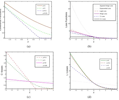
This proposition is depicted in Figure 1. Owing to the relationships of the

C

-lossCρ,1(y f(x))with the hinge and logit losses, it is potentially useful in devising new large-margin classifiers.

We now turn to the derivatives of Cρ,u(z) and(u−z)+. It is immediately verified that −1≤ C′_ρ_,_u(z)_≤0. Moreover, we have

lim

ρ→0C

′

ρ,u(z) =lim ρ→0V

′ ρ,u(z) =

  

0 z>u,

−1

2 z=u, −1 z<u.

Note that (u₋z)′₊ =₋1 ifz<u and(u₋z)′₊ =0 if z>u. Furthermore, ∂(u₋z)+|z=u= [−1,0]

where∂(u₋z)+|z=udenotes the subdifferential of(u−z)+ atz=u. Hence,

Proposition 5 For a fixed u>0, we have thatlimρ→0Cρ′,u(z)∈ ∂(u−z)+.

This proposition again establishes a connection of the hinge loss with the limit ofCρ,u(z) at

ρ=0. Furthermore, we obtain from Propositions 2 and 5 that ∂(u₋z)+ =∂limρ→0Cρ,u(z)∋

(9)

−1.5 −1 −0.5 0 0.5 1 1.5 2 0

0.5 1 1.5 2 2.5 3

z

Coherence Functions

ρ=2 ρ=1 ρ=0.1 ρ=0.01

−4 −3 −2 −1 0 1 2 3 4

0 5 10 15 20 25

z

Loss Functions

Squared Hinge Loss

Exponential Loss

Logit Loss

Hinge Loss

C−Loss

0−1 Loss

(a) (b)

−4 −3 −2 −1 0 1 2 3 4

0 0.5 1 1.5 2 2.5 3 3.5 4 4.5 5

z

C−losses

ρ=0.1 ρ=1 ρ=10 ρ=100

−4 −3 −2 −1 0 1 2 3 4

0 1 2 3 4 5 6

z

L−Losses

u=0

u=0.1

u=1

u=10

(c) (d)

Figure 1: These functions are regarded as a function ofz=y f(x). (a) Coherence functionsVρ,1(z) withρ=0.01,ρ=0.1, ρ=1 andρ=2. (b) A variety of majorization loss functions,

C-loss

: C1,1(z); Logit loss: L1,0(z); Exponential loss: exp(−z/2);Hinge loss: [1−z]+; Squared Hinge Loss:([1₋z]+)2. (c) Cρ,1(z)(orLρ,1(z)) withρ=0.1,ρ=1,ρ=10 and

ρ=100 (see Proposition 3-(i)). (d) L1,u(z)withu=0,u=0.1,u=1 andu=10 (see

Proposition 3-(ii)).

3.3 Consistency in Classification Methods

We now apply the coherence function to the development of classification methods. Recall that

C′_ρ_,_u(0) exists and is negative. Thus, the

C

-lossCρ,u(y f(x))is Fisher-consistent (or classification

calibrated) (Bartlett et al., 2006). In particular, we have the following theorem.

Theorem 6 Assume0<η<1andη₆=1

2. Consider the optimization problem min

(10)

for fixedρ>0and u≥0. Then, the minimizer is unique and is given by

f_∗(η) =ρlog

(2η₋1)exp(u

ρ) +

q

(1₋2η)2_exp₍2u

ρ) +4η(1−η)

2(1₋η) . (7)

Moreover, we have f_∗>0if and only ifη>1/2. Additionally, the inverse function f_∗−1(f)exists and it is given by

˜

η(f):= f_∗−1(f) = 1+exp(

f₋u

ρ )

1+exp(₋u+_ρf) +1+exp(f−_ρu), for f ∈R. (8)

The minimizer f_∗(x) of R(f(x)):=E(Vρ,u(Y f(X))|X =x) and its inverse ˜η(x) are

imme-diately obtained by replacing f with f(x) in (7) and (8). Since for u>0 the minimizers of

E(Cρ,u(Y f(X))|X=x)andE(Vρ,u(Y f(X))|X=x)are the same, this theorem shows thatCρ(y f(x),u)

is also Fisher-consistent. We see from Theorem 6 that the explicit expressions of f_∗(x)and its in-verse ˜η(x)exist. In the special case thatu=0, we have f_∗(x) =ρlog₁₋η(_ηx₍)_x₎and ˜η(x) = 1

1+exp(−f(x)/ρ).

Furthermore, whenρ=1, as expected, we recover logistic regression. In other words, the result is identical with that in Proposition 1 for logistic regression.

We further consider properties of f_∗(η). In particular, we have the following proposition.

Proposition 7 Let f_∗(η)be defined by (7). Then,

(i) sign(f_∗(η)) =sign(η₋1/2).

(ii) limρ→0f∗(η) =u×sign(η−1/2).

(iii) f_∗′(η) =d f∗(η)

dη ≥

ρ

η(1−η) with equality if and only if u=0.

Proposition 7-(i) shows that the classification rule with f_∗(x) is equivalent to the Bayes rule. In the special case that u=1, we have from Proposition 7-(ii) that limρ→0f∗(x) =sign(η(x)−

1/2). This implies that the current f_∗(x)approaches the solution ofE((1₋Y f(X))+|X=x), which

corresponds to the conventional SVM method (see Proposition 1).

We now treat ˜η(f)as a function ofρ. The following proposition is easily proven.

Proposition 8 Letη(˜ f)be defined by (8). Then, for fixed f _∈Rand u>0,limρ→∞η(˜ f) =1₂ and

lim

ρ→0η(˜ f) =           

1 if f >u, 2

3 if f =u, 1

2 if −u< f <u, 1

3 if f =−u, 0 if f <₋u.

As we discuss in the previous subsection, Vρ,u(z) is obtained when w=exp((u−z)/ρ)/(1+

exp((u₋z)/ρ))by using the maximum entropy principle. Let z=y f(x). We further write was

(11)

We now explore the relationship of ˜η(f)withw1(f)andw2(f). Interestingly, we first find that

˜

η(f) = w2(f) w1(f) +w2(f)

.

It is easily proven thatw1(f) +w2(f)≥1 with equality if and only if u=0. We thus have that ˜

η(f)_≤w2(f), with equality if and only ifu=0; that is, the loss becomes logit functionVρ,0(z). Note thatw2(f)represents the probability of the event{u+f >0}and ˜η(f)represents the probability of the event _{f >0_}. Since the event _{f >0_} is a subset of the event _{u+ f >0_}, we have

˜

η(f)_≤w2(f). Furthermore, the statement that ˜η(f) =w2(f) if and only ifu=0 is equivalent to {u+f >0_}=_{f >0_}if and only ifu=0. This implies that only the logit loss induces ˜η(f) = w2(f).

As discussed in Section 2.1, ˜η(x) can be regarded as a reasonable estimate of the true class probabilityη(x). Recall that_△R(η,f) =R(η,f)₋R(η,f_∗(η))and_△Rf =EX[△R(η(X),f(X))]

such that_△Rf can be viewed as the expected distance between ˜η(x)andη(x).

For an arbitrary fixed f ∈R, we have

△R(η,f) =R(η,f)₋R(η,f_∗(η)) =ηρlog 1+exp

u−f ρ

1+expu−f∗(η)

ρ

+ (1₋η)ρlog 1+exp

u+f ρ

1+expu+f∗(η)

ρ

.

The first-order derivative of_△R(η,f)with respect toηis

d_△R(η,f)

dη =ρlog

1+expu−_ρf

1+expu−f∗(η)

ρ

−ρlog 1+exp

u+f ρ

1+expu+f∗(η)

ρ

.

The Karush-Kuhn-Tucker (KKT) condition for the minimization problem is as follows:

η exp

u₋f_∗(η) ρ

1+expu−f∗(η)

ρ

+ (1₋η) exp

u+f_∗(η) ρ

1+expu+f∗(η)

ρ

=0,

and the second-order derivative of_△R(η,f)with respect toηis given by

d2△R(η,f)

dη2 =

1

1+exp(₋u−f∗(η)

ρ )

+ 1

1+exp(₋u+f∗(η)

ρ )

f_∗′(η) =

w1(f∗(η)) +w2(f∗(η))f∗′(η).

According to Proposition 7-(iii) and usingw1(f∗(η)) +w2(f∗(η))≥1, we have

d2_△R(η,f)

dη2 ≥

ρ η(1₋η),

with equality if and only if u=0. This implies d2△_dR_η(2η,f) >0. Thus, for a fixed f, △R(η,f) is

strictly convex inη. Subsequently, we have that_△R(η,f)_≥0 with equalityη=η˜, or equivalently,

(12)

Using the Taylor expansion of_△R(η,f)at ˜η:=η(˜ f) = f_∗−1(f), we thus obtain a lower bound for_△R(η,f); namely,

△R(η,f) =_△R(η˜,f)₋d△R(η˜,f)

dη (η−η) +˜

1 2

d2_△R(η¯,f)

dη2 (η−η)˜ 2

=1

2

d2_△R(η¯,f)

dη2 (η−η)˜

2_≥ ρ

2 ¯η(1₋η)¯ (η−η)˜

2_≥₂_ρ(η₋_η)_˜ 2_,

where ¯η_∈(η˜,η)_⊂[0,1]. In particular, we have that _△R(η,0) _≥2ρ(η₋0.5)2_{. According to} Theorem 2.1 and Corollary 3.1 in Zhang (2004), the following theorem is immediately established.

Theorem 9 Letε1=inff(·)∈FEX[△R(η(X),f(X))], and let f∗(x)∈

F

such that

EX[R(η(X),f∗(X))]≤ inf

f(·)∈FEX[R(η(X),f(X))] +ε2

forε2≥0. Then forε=ε1+ε2,

△Rf∗=EX[△R(η(X),f∗(X))]≤ε

and

Ψf∗≤Ψˆ + 2ε/ρ 1/2

,

whereΨf_∗ =EPI[Y f∗(X)≤0], andΨˆ =EPI[Y(2η(X)−1)≤0]is the optimal Bayes error. 3.4 Analysis

For notational simplicity, we will useCρ(z)forCρ,1(z). Considering f(x) =α+β′k, we define a regularized optimization problem of the form

min

α,β

n1

n

∑

i=1

Cρ(yif(xi)) +

γn

2β

′_K_βo

. (9)

Here we assume that the regularization parameterγrelies on the numbernof training data points, thus we denote it byγn.

Since the optimization problem (9) is convex with respect toαandβ, the solution exists and is unique. Moreover, sinceCρis infinitely smooth, we can resort to the Newton-Raphson method to

solve (9).

Proposition 10 Assume thatγnin (9) andγin (3) are same. Then the minimizer of (9) approaches

the minimizer of (3) asρ_→0.

This proposition is obtained directly from Proposition 5. For a fixedρ, we are also concerned with the universal consistency of the classifier based on (9) with and without the offset termα.

Theorem 11 Let K(_·,_·) be a universal kernel on

X

_×

X

. Suppose we are given such a positive sequence{γn}thatγn→0. If

nγ2_n/logn_→∞,

then the classifier based on (9) is strongly universally consistent. If

nγ2

n→∞,

(13)

Finally, we explore the convergence rate of the classification model in (9). It is worth point-ing out that Lin (2002) studied the convergence rate of theℓ2-SVM based on Theorem 4.1 in Lin (2000). Additionally, Lin (2002) argued that it is harder for the standard SVM to establish a similar convergence rate result due to two main reasons. The first one is that(1₋z)+is not differentiable

and the second one is that the target function sign(η₋1/2)is not in the assumed RKHS. We note that Theorem 4.1 in Lin (2000) is elaborated only for the least squares problem. It is also difficult to apply this theorem to our case, although the above two reasons no longer exist in our case. In Section 6.1 we illustrate how our classification model in (9) approaches the corresponding target function given in (7) using the same simulation data set as in Lin (2002). Moreover, under certain conditions, we can have the following theorem about convergence rate.

Theorem 12 Supposextakes values in a finite region with density p(x)and f(x) =α+h(x)with α taking values in a finite open interval. Assume that h belongs to a bounded open set of RKHS

H

_K with positive definite kernel K(_·,_·)and that there exists an M0>0such that|K(x1,x2)|<M0

if(x1,x2)are bounded. Letφ(z)be a strictly convex function and twice continuously differentiable.

We define

f∗ = argmin

f

Z

φ(y f(x))dF(x,y), ˆ

fn = argmin f

Z

φ(y f(x))dFn(x,y) +

γ

2khk 2 HK.

where F(x,y)is the distribution of(x,y)and Fn(x,y)is the empirical distribution of(x,y). Then we

have _Z

|fˆn(x)−f∗(x)|p(x)dx=O(γ) +Op(

1 √_n).

Obviously, the Gaussian RBF kernel satisfies the condition in Theorem 12. Since Cρ(z) is

strictly convex and infinitely smooth, we can directly apply Theorem 12 to the classification model in (9). In particular, let ˆfnbe the minimizer of Problem (9) and f∗(η)be defined in (7). Under the

conditions in Theorem 12, we have

Z

fˆ_n(x)−f_∗(η(x))

p(x)dx=O(γ) +O_p( 1 √

n).

4. Class Probability Estimation of SVM Outputs

As discussed earlier, the limit of the coherence function,Vρ,1(y f(x)), atρ=0 is just the hinge loss. Moreover, Proposition 7 shows that the minimizer ofVρ,1(f)η+Vρ,1(−f)(1−η)approaches that of

H(f)η+H(₋f)(1₋η)asρ_→0. Thus, Theorem 6 provides us with an approach to the estimation of the class probability for the conventional SVM.

In particular, let ˆf(x)be the solution of the optimization problem (3) for the conventional SVM. In terms of Theorem 6, we suggest that the estimated class probability ˆη(x)is defined as

ˆ

η(x) = 1+exp(

ˆ

f(x)−1

ρ )

1+exp(₋1+_ρfˆ(x)) +1+exp(fˆ(x_ρ)−1)

(14)

Proposition 7 would seem to motivate settingρto a very small value in (10). However, as shown in Proposition 8, the probabilistic outputs degenerate to 0, 1/3, 1/2, 2/3 and 1 in this case. Addi-tionally, the classification function ˆf(x) =αˆ+∑ni=1βˆiK(x,xi)is obtained via fitting a conventional

SVM model on the training data. Thus, rather than attempting to specify a fixed value of ρvia a theoretical argument, we instead view it as a hyperparameter to be fit empirically.

In particular, we fit ρ by minimizing the generalized Kullback-Leibler divergence (or cross-entropy error) between ˆη(X)andη(X), which is given by

GKL(η,η) =ˆ _EX

h

η(X)logη(X) ˆ

η(X)+ (1−η(X))log

1₋η(X)

1₋η(X)ˆ i

.

Alternatively, we formulate the optimization problem for obtainingρas

min

ρ>0 EKL(η)ˆ :=− 1

n

∑

i=1 n1

2(yi+1)log ˆη(xi) + 1

2(1−yi)log(1−η(ˆ xi)) o

. (11)

The problem can be solved by the Newton method. In summary, one first obtains ˆf(x) =αˆ + ∑ni=1βˆiK(x,xi) via the conventional SVM model, and estimates ρ via the optimization problem

in (11) based on the training data; one then uses the formula in (10) to estimate the class probabilities for the training samples as well as the test samples.

5.

C

-Learning

Focusing on the relationships of the

C

-lossCρ(y f(x)) (i.e.,Cρ,1(y f(x))) with the hinge and logit losses, we illustrate its application in the construction of large-margin classifiers. SinceCρ(y f(x))

is smooth, it does not tend to yield a sparse classifier. However, we can employ a sparsification penaltyJ(h)to achieve sparseness. We use the elastic-net penalty of Zou and Hastie (2005) for the experiments in this section. Additionally, we study two forms of f(x): kernel expansion and feature expansion. Built on these two expansions, sparseness can subserve the selection of support vectors and the selection of features, respectively. The resulting classifiers are called

C

-learning.

5.1 The Kernel Expansion

In the kernel expansion approach, given a reproducing kernelK(_·,_·):

X

_×

X

_→_R, we define the kernel expansion as f(x) =α+∑ni=1βiK(xi,x)and solve the following optimization problem:

min

α,β

1

n

∑

i=1

Cρ(yif(xi)) +γ

(1₋ω)1

2β

′_K_β₊_ω_k_β_k

1

, (12)

whereK= [K(xi,xj)]is then×nkernel matrix.

It is worth pointing out that the current penalty is slightly different from the conventional elastic-net penalty, which is(1₋ω)1

2β′β+ωkβk1. In fact, the optimization problem (12) can be viewed equivalently as the optimization problem

min

α,β

1

n

∑

i=1

Cρ(yif(xi)) +

γ

2β

(15)

under theℓ1penaltykβk1. Thus, the method derived from (12) enjoys the generalization ability of the conventional kernel supervised learning method derived from (13) but also the sparsity of theℓ1 penalty.

Recently, Friedman et al. (2010) devised a pathwise coordinate descent algorithm for regular-ized logistic regression problems in which the elastic-net penalty is used. In order to solve the optimization problem in (12), we employ this pathwise coordinate descent algorithm.

Let the current estimates of αandβ be ˆα and ˆβ. We first form a quadratic approximation to 1

n∑

n

i=1Cρ(yif(xi)), which is

Q(α,β) = 1

2nρ

n

∑

i=1

q(xi)(1−q(xi)) α+k′iβ−zi

2

+Const,

where

zi = αˆ+k′iβˆ+

ρ yi(1−q(xi))

,

q(xi) =

exp[(1₋yi(αˆ+k′iβ)ˆ /ρ]

1+exp[(1₋yi(αˆ +k′iβ))ˆ /ρ]

,

ki = (K(x1,xi), . . . ,K(xn,xi))′.

We then employ coordinate descent to solve the weighted least-squares problem as follows:

min

α,β

G(α,β):=Q(α,β) +γ(1₋ω)1

2β

′_K_β₊_ω_k_β_k

1

. (14)

Assume that we have estimated ˜β for βusing G(α,β). We now set ∂G(α, ˜

β)

∂α =0 to find the new

estimate ofα:

˜

α=∑

n

i=1q(xi)(1−q(xi)) zi−k′iβ˜

∑ni=1q(xi)(1−q(xi))

. (15)

On the other hand, assume that we have estimated ˜αforαand ˜βl forβl (l=1, . . . ,n,l6=j). We

now optimizeβj. In particular, we only consider the gradient atβj6=0. Ifβj>0, we have

∂G(α˜,β)˜ ∂βj

= 1 nρ

n

∑

i=1

Ki jq(xi)(1−q(xi)) α+k′iβ˜−zi

+γ(1₋ω)(Kj jβj+kjβ) +ˇ γω

and, hence,

˜

βj=

S(t₋γ(1₋ω)k′_jβˇ,γω)

1

nρ∑ni=1Ki j2q(xi)(1−q(xi)) +γ(1−ω)Kj j

, (16)

where t = 1

nρ∑ni=1Ki jq(xi)(1 − q(xi)) zi − α˜ − k′iβˇ

, βˇ = (β˜1, . . . ,β˜j−1,0,β˜j+1, . . . ,β˜n)′,

Ki j=K(xi,xj), andS(µ,ν)is the soft-thresholding operator:

S(µ,ν) =sign(µ)(_|µ| −ν)+

=

  

µ₋ν ifµ>0 andµ<_|ν_| µ+ν ifµ<0 andµ<_|ν_|

0 ifµ>_|ν_|.

(16)

Algorithm 1The coordinate descent algorithm for binary

C

-learning Input:

T

=_{xi,yi}n_i₌₁,γ,ω,εm,εi,ρ;

Initialize: α˜ =α0,β˜ =β0 repeat

CalculateG(α˜,β)˜ using (14);

α⋆_←α˜;

β⋆_←β˜; repeat

¯

α_←α˜; ¯

β_←β˜;

Calculate ˜αusing (15); for j=1tondo

Calculate ˜βj using (16);

end for

until_kα˜₋α¯_k+_kβ˜₋β¯_k<εi

until_kα˜₋α⋆_k₊_k_β˜₋_β⋆

k<εm

Output: α˜, ˜β, and f(x) =α˜+∑ni=1K(xi,x)β˜i.

5.2 The Linear Feature Expansion

In the linear feature expansion approach, we let f(x) =a+x′b, and pose the following optimization problem:

min

a,b 1

n

∑

i=1

Cρ(yif(xi)) +γJω(b), (17)

where forω_∈[0,1]

Jω(b) = (1−ω)

1 2kbk

2

2+ωkbk1=

d

∑

j=1 h1

2(1−ω)b 2

j+ω|bj|

i .

The elastic-net penalty maintains the sparsity of the ℓ1 penalty, but the number of variables to be selected is no longer bounded byn. Moreover, this penalty tends to generate similar coefficients for highly-correlated variables. We also use a coordinate descent algorithm to solve the optimization problem (17). The algorithm is similar to that for the kernel expansion and the details are omitted here.

6. Experimental Results

In Section 6.1 we illustrate convergence analysis of our classification method based on the

C

-loss. In Section 6.2 we report the results of experimental evaluations of our method for class probability estimation of the conventional SVM given in Section 4. In Section 6.3 we present results for the

C

-learning method given in Section 5.

6.1 Simulation Analysis for Convergence of

C

₋Learning

(17)

approaches the target function f_∗(η)given in (7) and how the class probability estimate ˜η(_fˆ_n₍_x₎₎_in (8) approaches the underlying class probabilityη(x).

For the purpose of visualization, we employ the same simulation data set as in Lin (2002). In particular, we taken equidistant points on the interval[0,1]; that is, xi= (i−1)/nfori=1, . . . ,n.

Let η(x) =Pr(Y =1_|X =x) =1_{− |}1₋2x_|. Then the target function f_∗(η(x)) for our model is computed by (7). We randomly generateyito be 1 or−1 with probabilityη(xi)and 1−η(xi), and

form a training data set _{(xi,yi);i=1. . . ,n}. Following the setting in Lin (2002), we implement

our simulations on RKHS

H

m_([₀_,₁_])_{(i.e., the Sobolev Hilbert space with order} _m _{of univariate}

functions on domain[0,1]) and four data sets with sizen=33, 65, 129 and 257. The parameters

γ andρ are chosen to minimize the generalized KL (GKL) divergence by the grid search. The implementation is based on the

C

-learning algorithm in Section 5 where the hyperparameter ωis approximately set as 0.

Figures 2 and 3 respectively depict the solutions ˆfnto the regularization problem in (9) and the

class probability estimates ˜η(_fˆ_n₎_{given in (8), when the sample size is}_n₌_{33, 65, 129, and 257. We} can see that the solution ˆfnis close the target function f∗(η)and that the class probability estimate

˜

η(fˆn) is close the underlying class probability η, as n increases. Thus, our simulation example

shows that our method based on

C

-loss not only can approach its corresponding target function

f_∗(η)but also can estimate the underlying class probabilityη(x). It should be pointed out that the similar experimental results can be found on the Gaussian RBF kernel, so here we do not include the results with the Gaussian RBF kernel.

6.2 Simulation for Class Probability Estimation of SVM Outputs

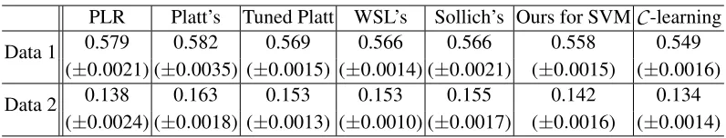
We validate our estimation method for the class probability of SVM outputs (“Ours for SVM”), comparing it with several alternatives: Platt’s method (Platt, 1999), Sollich’s method (Sollich, 2002), and the method of Wang et al. (2008) (WSL’s). Since penalized (or regularized) logistic regression (PLR) and

C

-learning can directly calculate class probability, we also implement them. Especially, the class probability of

C

-learning outputs is based on (8) where we setρ=1 andu=1 since

C

-learning itself employs the same setting.

We conducted our analysis over two simulation data sets which were used by Wang et al. (2008). The first simulation data set,_{(xi1,xi2;yi)}1000i=1 , was generated as follows. The{(xi1,xi2)}1000i=1 were uniformly sampled from a unit disk _{(x1,x2):x2₁+x2₂ ≤1}. Next, we setyi=1 if xi1 ≥0 and

yi =−1 otherwise, i=1, . . . ,1000. Finally, we randomly chose 20% of the samples and flipped

their labels. Thus, the true class probabilityη(Yi=1|xi1,xi2)was either 0.8 or 0.2.

The second data set, _{(xi1,xi2;yi)}1000_i₌1 , was generated as follows. First, we randomly assigned 1 or₋1 toyi fori=1, . . . ,1000 with equal probability. Next, we generatedxi1from the uniform distribution over[0,2π], and setxi2=yi(sin(xi1) +εi) whereεi∼N(εi|1,0.01). For the data, the

true class probability ofY =1 was given by

η(Y =1_|x1,x2) =

N(x2|sin(x1)+1,0.01)

N(x2|sin(x1)+1,0.01) +N(x2| −sin(x1)−1,0.01) .

(18)

0 0.2 0.4 0.6 0.8 1 0

0.1 0.2 0.3 0.4 0.5 0.6 0.7 0.8 0.9 1

X

Class Probability

η(x) ˜

η(x)

0 0.2 0.4 0.6 0.8 1

0 0.1 0.2 0.3 0.4 0.5 0.6 0.7 0.8 0.9 1

X

Class Probability

η(x) ˜

η(x)

(a)n=33,γ=5.9186_×10−5_,_ρ₌₀_.₅₆₉₅ _(b)_n₌_65,_γ₌₇_.₅₁₂₀_×₁₀−6_,_ρ₌₀_.₅₆₉₅

0 0.2 0.4 0.6 0.8 1

0 0.1 0.2 0.3 0.4 0.5 0.6 0.7 0.8 0.9 1

X

Class Probability

η(x) ˜

η(x)

0 0.2 0.4 0.6 0.8 1

0 0.1 0.2 0.3 0.4 0.5 0.6 0.7 0.8 0.9 1

X

Class Probability

η(x) ˜

η(x)

(c)n=129,γ=1.5141_×10−5,ρ=0.5695 (d)n=257,γ=3.7999_×10−6,ρ=0.5695 Figure 2: The underlying class probabilitiesη(x)(“blue + dashed line”) and estimated class

proba-bilities ˜η(x) =η(˜ fˆn(x))(“red + solid line”) on RKHS

H

m([0,1])and the simulation data

sets with the sizen=33, 65, 129, and 257. Here the values of parametersγandρin each data set are obtained by minimizing the GKL divergence.

employed a Gaussian RBF kernelK(xi,xj) =exp(−kxi−xjk2/σ2)where the parameterσwas set

as the median distance between the positive and negative classes. We reported GKL and CER as well as the corresponding standard deviations in Tables 2 and 3 in which the results with the PLR method, the tuned Platt method and the WSL method are directly cited from Wang et al. (2008).

(19)

0 0.2 0.4 0.6 0.8 1 −4

−3 −2 −1 0 1 2 3

X

Decision Function

f⋆(η)

ˆ

fn

0 0.2 0.4 0.6 0.8 1

−3 −2 −1 0 1 2 3

X

Decision Function

f⋆(η)

ˆ

fn

(a)n=33,γ=5.9186_×10−5_,_ρ₌₀_.₅₆₉₅ _(b)_n₌_65,_γ₌₇_.₅₁₂₀_×₁₀−6_,_ρ₌₀_.₅₆₉₅

0 0.2 0.4 0.6 0.8 1

−4 −3 −2 −1 0 1 2 3 4

X

Decision Function

f⋆(η)

ˆ

fn

0 0.2 0.4 0.6 0.8 1

−4 −3 −2 −1 0 1 2 3 4

X

Decision Function

f⋆(η)

ˆ

fn

(c)n=129,γ=1.5141_×10−5,ρ=0.5695 (d)n=257,γ=3.7999_×10−6,ρ=0.5695 Figure 3: The target decision functionf_∗(η)(“blue + dashed line”) and estimated decision functions

ˆ

fn(“red + solid line”) on RKHS

H

m([0,1])and the toy data sets with the sizen=33, 65,

129, and 257. The parameters are identical to the settings in Figure 2.

probability outputs. In other words, ˆη(x)>1/2 is not equivalent to ˆf(x)>0 for Platt’s method. In fact, Platt (1999) used the sigmoid-like function to improve the classification accuracy of the conventional SVM. As for the method of Wang et al. (2008) which is built on a sequence of weighted classifiers, the CERs of the method should be different from those of the original SVM. With regard to CER, the performance of PLR is the worst in most cases.

6.3 The Performance Analysis of

C

-Learning

(20)

PLR Platt’s Tuned Platt WSL’s Sollich’s Ours for SVM

C

-learning

Data 1 0.579 0.582 0.569 0.566 0.566 0.558 0.549 (_±0.0021) (_±0.0035) (_±0.0015) (_±0.0014) (_±0.0021) (_±0.0015) (_±0.0016)

Data 2 0.138 0.163 0.153 0.153 0.155 0.142 0.134 (_±0.0024) (_±0.0018) (_±0.0013) (_±0.0010) (_±0.0017) (_±0.0016) (_±0.0014)

Table 2: Values of GKL over the two simulation test sets (standard deviations are shown in paren-theses).

PLR Platt’s WSL’s Ours for SVM

C

-learning

Data 1 0.258 0.234 0.217 0.219 0.214 (_±0.0053) (_±0.0026) (_±0.0021) (_±0.0021) (_±0.0015)

Data 2 0.075 0.077 0.069 0.065 0.061 (_±0.0018) (_±0.0024) (_±0.0014) (_±0.0015) (_±0.0019)

Table 3: Values of CER over the two simulation test sets (standard deviations are shown in paren-theses).

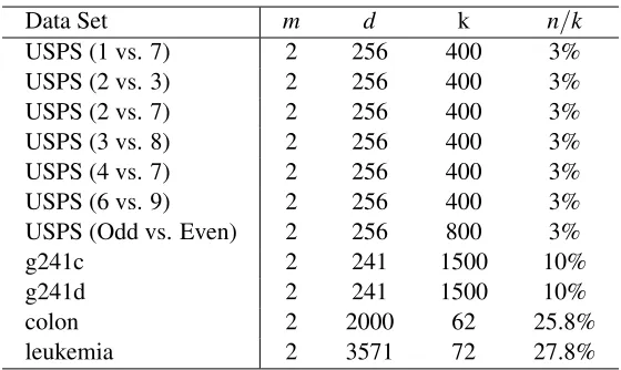
In the experiments we used 11 binary classification data sets. Table 4 gives a summary of these benchmark data sets. The seven binary data sets of digits were obtained from the publicly available USPS data set of handwritten digits as follows. The first six data sets were generated from the digit pairs_{(1, 7), (2, 3), (2, 7), (3, 8), (4, 7), (6,9)_}, and 200 digits were chosen within each class of each data set. The USPS (odd vs. even) data set consisted of the first 80 images per digit in the USPS training set.

The two binary artificial data sets of “g241c” and “g241d” were generated via the setup pre-sented by Chapelle et al. (2006). Each class of these two data sets consisted of 750 samples.

The two binary gene data sets of “colon” and “leukemia” were also used in our experiments. The “colon” data set, consisting of 40 colon tumor samples and 22 normal colon tissue samples with 2,000 dimensions, was obtained by employing an Affymetrix oligonucleotide array to analyze more than 6,500 human genes expressed in sequence tags (Alon et al., 1999). The “leukemia” data set is of the same type as the “colon” cancer data set (Golub et al., 1999), and it was obtained with respect to two variants of leukemia, that is, acute myeloid leukemia (AML) and acute lymphoblastic leukemia (ALL). It initially contained expression levels of 7129 genes taken over 72 samples (AML, 25 samples, or ALL, 47 samples), and then it was pre-feature selected, leading to a feature space with 3571 dimensions.

In our experiments, each data set was randomly partitioned into two disjoint subsets as the training and test, with the percentage of the training data samples also given in Table 4. Twenty random partitions were chosen for each data set, and the average and standard deviation of their classification error rates over the test data were reported.

(21)

Data Set m d k n/k

USPS (1 vs. 7) 2 256 400 3% USPS (2 vs. 3) 2 256 400 3% USPS (2 vs. 7) 2 256 400 3% USPS (3 vs. 8) 2 256 400 3% USPS (4 vs. 7) 2 256 400 3% USPS (6 vs. 9) 2 256 400 3% USPS (Odd vs. Even) 2 256 800 3%

g241c 2 241 1500 10%

g241d 2 241 1500 10%

colon 2 2000 62 25.8%

leukemia 2 3571 72 27.8%

Table 4: Summary of the benchmark data sets:m—the number of classes;d—the dimension of the input vector;k—the size of the data set;n—the number of the training data.

Data Set HHSVM RLRM

C

-learning (1 vs. 7) 2.29_±1.17 2.06_±1.21 1.60_±0.93 (2 vs. 3) 8.13_±2.02 8.29_±2.76 8.32_±2.73 (2 vs. 7) 5.82_±2.59 6.04_±2.60 5.64_±2.44 (3 vs. 8) 12.46_±2.90 10.77_±2.72 11.74_±2.83 (4 vs. 7) 7.35_±2.89 6.91_±2.72 6.68_±3.53 (6 vs. 9) 2.32_±1.65 2.15_±1.43 2.09_±1.41 (Odd vs. Even) 20.94_±2.02 19.83_±2.82 19.74_±2.81 g241c 22.30±1.30 21.38±1.12 21.34_±1.11 g241d 24.32_±1.53 23.81_±1.65 23.85_±1.69 colon 14.57_±1.86 14.47_±2.02 12.34_±1.48 leukemia 4.06_±2.31 4.43_±1.65 3.21_±1.08

Table 5: Classification error rates (%) and standard deviations on the 11 data sets for the feature expansion setting.

the relationship of the

C

-lossC(z)with the hinge loss(1₋z)+and the logit loss log(1+exp(−z))

(see our analysis in Section 3 and Figure 1).

As for the parametersγandω, they were selected by cross-validation for all the classification methods. In the kernel expansion, the RBF kernelK(xi,xj) =exp(−kxi−xjk2/σ2)was employed,

andσwas set to the mean Euclidean distance among the input samples. For

C

-learning, the other parameters were set as follows:εm=εi=10−5.

Tables 5 and 6 show the test results corresponding to the linear feature expansion and RBF kernel expansion, respectively. From the tables, we can see that for the overall performance of

C

-learning is slightly better than the two competing methods in the feature and kernel settings generally.

(22)

Data Set HHSVM RLRM

C

-learning (1 vs. 7) 1.73_±1.64 1.39_±0.64 1.37_±0.65 (2 vs. 3) 8.55_±3.36 8.45_±3.38 8.00_±3.32 (2 vs. 7) 5.09_±2.10 4.02_±1.81 3.90_±1.79 (3 vs. 8) 12.09_±3.78 10.58_±3.50 10.36_±3.52 (4 vs. 7) 6.74_±3.39 6.92_±3.37 6.55_±3.28 (6 vs. 9) 2.12_±0.91 1.74_±1.04 1.65_±0.99 (Odd vs. Even) 28.38_±10.51 26.92_±6.52 26.29_±6.45 g241c 21.38_±1.45 21.55_±1.42 21.62_±1.35 g241d 25.89_±2.15 22.34_±1.27 20.37_±1.20 colon 14.26_±2.66 14.79_±2.80 13.94_±2.44 leukemia 2.77_±0.97 2.74_±0.96 2.55_±0.92

Table 6: Classification error rates (%) and standard deviations on the 11 data sets for the RBF kernel setting.

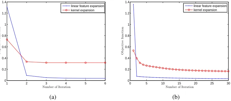
the objective function for the data set USPS (1 vs. 7) similar results were found on all other data sets. This shows that the coordinate descent algorithm is very efficient.

We also conducted a systematic study of sparseness from the elastic-net penalty. Indeed, the elastic-net penalty does give rise to sparse solutions for our

C

-learning methods. Moreover, we found that similar to other methods the sparseness of the solution is dependent on the parametersγ

andωthat were set to different values for different data sets using cross validation.

1 2 3 4 5 6

0 0.2 0.4 0.6 0.8 1 1.2 1.4

O

b

je

c

ti

v

e

fu

n

c

ti

o

n

Number of Iteration

linear feature expansion kernel expansion

0 5 10 15 20 25 30

0 0.2 0.4 0.6 0.8 1 1.2 1.4

Number of Iteration

O

b

je

c

ti

v

e

fu

n

c

ti

o

n

linear feature expansion kernel expansion

(a) (b)

(23)

7. Conclusions

In this paper we have studied a family of coherence functions and considered the relationship be-tween coherence functions and hinge functions. In particular, we have established some important properties of these functions, which lead us to a feasible approach for class probability estimation in the conventional SVM. Moreover, we have proposed large-margin classification methods using the

C

-loss function and the elastic-net penalty, and developed pathwise coordinate descent algorithms for parameter estimation. We have theoretically established the Fisher-consistency of our classifica-tion methods and empirically tested the classificaclassifica-tion performance on several benchmark data sets. Our approach establishes an interesting link between SVMs and logistic regression models due to the relationship of the

C

-loss with the hinge and logit losses.

Acknowledgments

The authors would like to thank the Action Editor and three anonymous referees for their construc-tive comments and suggestions on the original version of this paper. This work has supported in part by the Natural Science Foundations of China (No. 61070239), the US ARL and the US ARO under contract/grant number W911NF-11-1-0391.

Appendix A. The Proof of Proposition 2

First, we have

ρlog 2+ [u₋z]+−Vρ,u(z) =ρlog

2 exp[u−z]+ ρ

1+expu−_ρz ≥0.

Second, note that

ρlog 2+u−z

2 −Vρ,u(z) =ρlog

2 exp1₂u−_ρz 1+expu−_ρz

≤ρlog exp

u₋z ρ

1+expu−_ρz ≤0,

where we use the fact that exp(_·)is convex.

Third, it immediately follows from Proposition (i) that limρ_→0Vρ,u(z) = [u−z]+. Moreover, it

is easily obtained that

lim

ρ→∞Vρ,u(z)−ρlog 2=ρlim→∞

log1+exp

u−z

ρ

2 1

ρ

=lim

α→0

log1+exp₂α(u−z)

α

=lim

α→0 1

2[u−z]exp[α(u−z)] 1+expα(u−z)

2

=1

2(u−z).

Since log(1+a)_≥log(a)fora>0, we have

u

log[1+exp(u/ρ)]log

1+expu−z

ρ

≤_u_/u_ρlog1+expu−z

ρ

=ρlog1+expu−z

ρ

(24)

We now consider that

lim

ρ→∞Cρ,u(z) =uρlim→∞

logh1+expu−_ρzi log[1+exp(u/ρ)] =u.

Finally, since

lim

α→∞

log[1+exp(uα)]

αu =αlim→∞

exp(uα)]

1+exp(uα) =1 for u>0,

we obtain limρ→0Cρ,u(z) = [u−z]+.

Appendix B. The Proof of Proposition 3

Before we prove Proposition 3, we establish the following lemma.

Lemma 13 Assume that x>0, then f1(x) =₁₊x_x_loglog₍₁₊x_x₎and f2(x) =₁₊x_x_log₍1₁₊_x₎are increasing and

decreasing, respectively.

Proof The first derivatives of f1(x)and f2(x)are

f₁′(x) = 1

(1+x)2_log2₍₁₊_x) h

logxlog(1+x) +log(1+x) +xlog(1+x)₋xlogx

i

f₂′(x) = 1

(1+x)2_log2₍₁₊_x)[log(1+x)−x]≤0.

This implies that f2(x)is decreasing. If logx≥0, we havexlog(1+x)−xlogx≥0. Otherwise, if logx<0, we have logx[log(1+x)₋x]_≥0. This implies that f₁′(x)_≥0 is always satisfied. Thus,

f1(x)is increasing.

Let α=1/ρ and use h1(α) for Lρ,u(z) to view it as a function ofα. We now compute the

derivative ofh1(α)w.r.t.α:

h′₁(α) = log[1+exp(α(u−z))]

log[1+exp(uα)] ×

h exp(α(u−z)) 1+exp(α(u₋z))

u₋z

log[1+exp(α(u₋z))]−

exp(αu)

1+exp(αu)

u

log[1+exp(αu)]

i

= log[1+exp(α(u−z))] αlog[1+exp(uα)] ×

log exp(α(u₋z))

exp(αu)

1+exp(αu)

log exp(αu)

log[1+exp(αu)]

i .

Whenz<0, we have exp(α(u₋z))>exp(αu). It then follows from Lemma 13 that h′₁(α)_≥0. Whenz_≥0, we haveh′₁(α)_≤0 due to exp(α(u₋z))_≤exp(αu). The proof of (i) is completed.

To prove part (ii), we regard Lρ,u(z) as a function of u and denote it with h2(u). The first derivativeh′₂(u)is given by

h′₂(u) = αlog[1+exp(α(u−z))]

log[1+exp(uα)] ×

1

exp(αu)

1+exp(αu)

1 log[1+exp(αu)]

(25)

Using Lemma 13, we immediately obtain part (ii).

Appendix C. The Proof of Theorem 6

We write the objective function as

L(f) =Vρ,u(f)η+Vρ,u(−f)(1−η)

=ρlog1+expu−f

ρ

η+ρlog1+expu+f

ρ

(1₋η).

The first-order and second-order derivatives ofLw.r.t. f are given by

dL d f =−η

expu−_ρf

1+expu−_ρf + (1−η)

expu+_ρf

1+expu+_ρf ,

d2L d f2 =

η ρ

expu−_ρf

1+expu−_ρf 1

1+expu−_ρf + 1₋η

ρ

expu+_ρf

1+expu+_ρf 1

1+expu+_ρf.

Since d_{d f}2L2 >0, the minimum ofLis unique. Moreover, letting dL

d f =0 yields (7).

Appendix D. The Proof of Proposition 7

First, ifη>1/2, we have 4η(1₋η)>4(1₋η)2_and₍₂_η₋₁₎_exp_(u_/_ρ)_>_{0. This implies} _f

∗>0.

Whenη<1/2, we have(2η₋1)exp(u/ρ)>0. In this case, since

(1₋2η)2exp(2u/ρ) +4η(1₋η)<(1₋2η)2exp(2u/ρ) +4(1₋η)2+4(1₋η)(1₋2η)exp(u/ρ), we obtain f_∗<0.

Second, lettingα=1/ρ, we express f_∗as

f_∗= 1 αlog

(2η₋1)exp(uα) +p(1₋2η)2_exp₍₂_{uα) +}₄_η(₁₋_η) 2(1₋η)

= 1 αlog

(2η−1)

|2η−1|+

q

1+₍₁ 4η(1−η)

−2η)2_exp₍₂_u_α₎

2(1₋η)exp(₋uα)/_|2η₋1_|

= 1 αlog

"

(2η₋1)

|2η₋1_| + s

1+ 4η(1−η) (1₋2η)2_exp₍₂_uα)

#

−_α1log

h2(1−η) |2η₋1_|

i

+u.

Thus, ifη>1/2, it is clear that limα→∞f∗=u. In the case thatη<1/2, we have

lim

α→∞f∗=u−uαlim→∞

1

−1+q1+₍₁ 4η(1−η)

−2η)2_exp₍₂_u_α₎

1 q

1+₍₁ 4η(1−η)

−2η)2_exp₍₂_u_α₎

4η(1₋η)

(1₋2η)2 exp(−2uα)

=u₋4η(1−η)u (1₋2η)2 _αlim_→_∞

exp(₋2uα)

−1+q1+₍₁ 4η(1−η)

−2η)2_exp₍₂_u_α₎

=u₋2ulim

α→∞

s

1+ 4η(1−η) (1₋2η)2_exp₍₂_uα)

(26)

Here we use l’Hˆopital’s rule in calculating limits.

Third, letα=exp(u/ρ). It is then immediately calculated that

f_∗′(η) =2ρ

α+√ (1−2η)(1−α2)

(1−2η)2_α2₊₄_η₍₁₋_η₎

(2η₋1)α+p(1₋2η)2_α2₊₄_η(₁₋_η)+

ρ

1−η.

Consider that

A=

2α+√ 2(1−2η)(1−α2)

(1−2η)2_α2₊₄_η₍₁₋_η₎

(2η₋1)α+p(1₋2η)2_α2₊₄_η(₁₋_η)− 1

η

=

α₋√ 2η+(1−2η)α2

(1₋2η)2_α2₊₄_η₍₁₋_η₎

η(2η₋1)α+ηp(1₋2η)2_α2₊₄_η(₁₋_η). It suffices for f_∗′(η)_≥_η₍₁ρ₋_η₎to showA_≥0. Note that

(2η+ (1₋2η)α2₎2

(1₋2η)2_α2₊₄_η(₁₋_η)−α

2₌ 4η2(1−α2)

(1₋2η)2_α2₊₄_η(₁₋_η)≤0

due toα_≥1, with equality when and only when α=1 or, equivalently, u=0. Accordingly, we haveα₋√ 2η+(1−2η)α2

(1−2η)2_α2₊₄_η₍₁₋_η₎≥0.

Appendix E. The Proof of Theorem 11

In order to prove the theorem, we define

δγ:=sup{t:γt2≤2Vρ(0)}=

p 2/γ

forγ>0 and letVρ(γ)(y f)be the coherence functionVρ(y f)restricted to

Y

×[−δγkmax,δγkmax], where

kmax=maxx∈XK(x,x). For the Gaussian RBF kernel, we havekmax=1. It is clear that

kVρ(γ)k∞:=supVρ(γ)(y f),(y,f)∈

Y

×[−δγkmax,δγkmax] =ρlog

1+expu+kmax p

2/γ ρ

.

Considering that

lim

γ→0

kVρ(γ)k∞

kmax p

2/γ=αlim→∞

expu+_ρα

1+expu+_ρα =1,

we have limγ→0kVρ(γ)k∞/

p

1/γ=√2kmax. Hence, we have_kVρ(γ)k∞∼

p 1/γ. On the other hand, since

Vρ(γ)(y f) =Vρ(γ)(y f1)−

∂Vρ(γ)(y f2)

(27)

where f2∈[f,f1]⊆[−δγkmax,δγkmax], we have

|Vρ(γ)|1:=sup (

|Vρ(γ)(y f)−Vρ(γ)|(y f1) |f₋f1|

,y_∈

Y

,f,f1∈[−δγkmax,δγkmax],f6= f1 )

=sup (

∂Vρ(γ)(y f2)

∂f

,y∈

Y

,f2∈[−δγkmax,δγkmax] )

= exp

u+kmax√2/γ ρ

1+expu+kmax√2/γ ρ

.

In this case, we have limγ→0|Vρ(γ)|1=1, which implies that|Vρ(γ)|1∼1.

We now immediately conclude Theorem 11 from Corollary 3.19 and Theorem 3.20 of Steinwart (2005).

Appendix F. The Proof of Theorem 12

Note that the condition for function in the theorem implies thatφ′′_(z)_>_{0 in}_R_{, then it follows that}

φ′′(z)>δfor some positiveδin a compact region (and certainly also holds in any bounded region). We also denote

¯

fn=argmin f

Z

φ(y f(x))dFn(x,y)

and

L(f) = Z

φ(y f(x))dF(x,y),

Ln1(f) =

Z

φ(y f(x))dFn(x,y) +

γ

2khk 2 HK,

Ln2(f) =

Z

φ(y f(x))dFn(x,y).

We have f∗,_f¯_n_,_fˆ_n_{are all unique, because the corresponding objective functions are strictly convex.} Taking the derivative of the functionalL(f)w.r.t. f yields

Z

yvφ′(y f∗)dF(x,y) =0 for anyv_∈