Classification Using Geometric Level Sets
Kush R. Varshney [email protected]
Alan S. Willsky [email protected]
Laboratory for Information and Decision Systems Massachusetts Institute of Technology
Cambridge, MA 02139-4309, USA
Editor: Ulrike von Luxburg
Abstract
A variational level set method is developed for the supervised classification problem. Nonlinear classifier decision boundaries are obtained by minimizing an energy functional that is composed of an empirical risk term with a margin-based loss and a geometric regularization term new to machine learning: the surface area of the decision boundary. This geometric level set classifier is analyzed in terms of consistency and complexity through the calculation of itsε-entropy. For multicategory classification, an efficient scheme is developed using a logarithmic number of decision functions in the number of classes rather than the typical linear number of decision functions. Geometric level set classification yields performance results on benchmark data sets that are competitive with well-established methods.
Keywords: level set methods, nonlinear classification, geometric regularization, consistency, com-plexity
1. Introduction
Variational level set methods, pioneered by Osher and Sethian (1988), have found application in fluid mechanics, computational geometry, image processing and computer vision, computer graph-ics, materials science, and numerous other fields, but have heretofore found little application in machine learning. The goal of this paper is to introduce a level set approach to the archetypal ma-chine learning problem of supervised classification. We propose an implicit level set representation for classifier decision boundaries, a margin-based objective regularized by a surface area penalty, and an Euler-Lagrange descent optimization algorithm for training.
Several well-developed techniques for supervised discriminative learning exist in the literature, including the perceptron algorithm (Rosenblatt, 1958), logistic regression (Efron, 1975), and sup-port vector machines (SVMs) (Vapnik, 1995). All of these approaches, in their basic form, produce linear decision boundaries. Nonlinear boundaries in the input space can be obtained by mapping the input space to a feature space of higher (possibly infinite) dimension by taking nonlinear functions of the input variables. Learning algorithms are then applied to the new higher-dimensional feature space by treating each dimension linearly. They retain the efficiency of the input lower-dimensional space for particular sets of nonlinear functions that admit the kernel trick (Sch¨olkopf and Smola, 2002).
clas-dimensional surface in a three-clas-dimensional space, and generally a D−1 dimensional hypersurface in a D-dimensional space. Classifier decision boundaries partition the input space into regions cor-responding to the different class labels. If the region corcor-responding to one class label is composed of several unconnected pieces, then the corresponding decision boundary is composed of several un-connected pieces; we refer to this entire collection of decision boundaries as the contour. The level set representation is a flexible, implicit representation for contours that does not require knowing the number of disjoint pieces in advance. The contour is represented by a smooth, Lipschitz contin-uous, scalar-valued function, known as the level set function, whose domain is the input space. The contour is implicitly specified as the zero level set of the level set function.
Level set methods entail not only the representation, but also the minimization of an energy
functional whose argument is the contour.1 For example, in foreground-background image
seg-mentation, a popular energy functional is mean squared error of image intensity with two different ‘true’ image intensities inside the contour and outside the contour. Minimizing this energy produces a good segmentation when the two regions differ in image intensity. In order to perform the min-imization, a gradient descent approach is used. The first variation of the functional is found using the calculus of variations; starting from an initial contour, a gradient flow is followed iteratively to converge to a minimum. This procedure is known as curve evolution or contour evolution.
The connection between level set methods (particularly for image segmentation) and classifica-tion has been noticed before, but to the best of our knowledge, there has been little prior work in this area. Boczko et al. (2006) only hint at the idea of using level set methods for classification. Tom-czyk and Szczepaniak (2005) do not consider fully general input spaces. Specifically, examples in the training and test sets must be pixels in an image with the data vector containing the spatial index of the pixel along with other variables. Cai and Sowmya (2007) do consider general feature spaces, but have a very different energy functional than our margin-based loss functional. Theirs is based on counts of training examples in grid cells and is similar to the mean squared error functional for image segmentation described earlier. Their learning is also based on one-class classification rather than standard discriminative classification, which is the framework we follow. Yip et al. (2006) use variational level set methods for density-based clustering in general feature spaces, rather than for learning classifiers.
Cremers et al. (2007) dichotomize image segmentation approaches into those that use spatially continuous representations and those that use spatially discrete representations, with level set meth-ods being the main spatially continuous approaches. There have been methmeth-ods using discrete rep-resentations that bear some ties to our methods. An example of a spatially discrete approach uses normalized graph cuts (Shi and Malik, 2000), a technique that has been used extensively in unsu-pervised learning for general features unrelated to images as well. Normalized decision boundary surface area is implicitly penalized in this discrete setting. Geometric notions of complexity in
pervised classification tied to decision boundary surface area have been suggested by Ho and Basu (2002), but also defined in a discrete way related to graph cuts. In contrast, the continuous formula-tion we employ using level sets involves very different mathematical foundaformula-tions, including explicit minimization of a criterion involving surface area. Moreover, the continuous framework—and in particular the natural way in which level set functions enter into the criterion—lead to new gradient descent algorithms to determine optimal decision boundaries. By embedding our criterion in a con-tinuous setting, the surface area complexity term is defined intrinsically rather than being defined in terms of the graph of available training examples.
There are some other methods in the literature for finding nonlinear decision boundaries directly in the input space related to image segmentation, but these methods use neither contour evolution for optimization, nor the surface area of the decision boundary as a complexity term, as in the level set classification method proposed in this paper. A connection is drawn between classification and level set image segmentation in Scott and Nowak (2006) and Willett and Nowak (2007), but the formulation is through decision trees, not contour evolution. Tomczyk (2005), Tomczyk and Szczepaniak (2006), and Tomczyk et al. (2007) present a simulated annealing formulation given the name adaptive potential active hypercontours for finding nonlinear decision boundaries in both the classification and clustering problems; their work considers the use of radial basis functions in representing the decision boundary. P¨olzlbauer et al. (2008) construct nonlinear decision boundaries in the input space from connected linear segments. In some ways, their approach is similar to active contours methods in image segmentation such as snakes that do not use the level set representation: changes in topology of the decision boundary in the optimization are difficult to handle. (The implicit level set representation takes care of topology changes naturally.)
The theory of classification with Lipschitz functions was discussed by von Luxburg and Bous-quet (2004). As mentioned previously, level set functions are Lipschitz functions and the spe-cific level set function that we use, the signed distance function, has a unit Lipschitz constant. Von Luxburg and Bousquet minimize the Lipschitz constant, whereas in our formulation, the Lip-schitz constant is fixed. The von Luxburg and Bousquet formulation requires the specification of a subspace of Lipschitz functions over which to optimize in order to prevent overfitting, but does not resolve the question of how to select this subspace. The surface area penalty that we propose provides a natural specification for subspaces of signed distance functions.
The maximum allowable surface area parameterizes nested subspaces. We calculate the ε
-entropy (Kolmogorov and Tihomirov, 1961) of these signed distance function subspaces and use the result to characterize geometric level set classification theoretically. In particular, we look at the consistency and convergence of level set classifiers as the size of the training set grows. We also look at the Rademacher complexity (Koltchinskii, 2001; Bartlett and Mendelson, 2002) of level set classifiers.
For the multicategory classification problem with M>2 classes, typically binary classification
methods are extended using the all construction (Hsu and Lin, 2002). The one-against-all scheme represents the classifier with M decision functions. We propose a more parsimonious
representation of the multicategory level set classifier that uses log2M decision functions.2 A
col-lection of log2M level set functions can implicitly specify M regions using a binary encoding like
a Venn diagram (Vese and Chan, 2002). This proposed logarithmic multicategory classification is
Repository and find the results to be competitive with many classifiers used in practice.
Level set methods are usually implemented on a discretized grid, that is the values of the level set function are maintained and updated on a grid. In physics and image processing applications, it nearly always suffices to work in two- or three-dimensional spaces. In classification problems, however, the input data space can be high-dimensional. Implementation of level set methods for large input space dimension becomes cumbersome due to the need to store and update a grid of that large dimension. One way to address this practical limitation is to represent the level set function by a superposition of radial basis functions (RBFs) instead of on a grid (Cecil et al., 2004; Slabaugh et al., 2007; Gelas et al., 2007). We follow this implementation strategy in obtaining classification results.
In Section 2, we detail geometric level set classification in the binary case, giving the objective to be minimized and the contour evolution to perform the minimization. In Section 3, we pro-vide theoretical analysis of the binary level set classifier given in Section 2. The main result is
the calculation of theε-entropy of the space of level set classifiers as a function of the maximum
allowable decision boundary surface area; this result is then applied to characterize consistency and complexity. Section 4 goes over multicategory level set classification. In Section 5, we describe the RBF level set implementation and use that implementation to compare the classification test perfor-mance of geometric level set classification to the perforperfor-mance of several other classifiers. Section 6 concludes and provides a summary of the work.
2. Binary Geometric Level Set Classification
In the standard binary classification problem, we are given training data {(x1,y1), . . . ,(xn,yn)}
with data vectors xi∈Ω⊂RDand class labels yi∈ {+1,−1}drawn according to some unknown
probability density function pX,Y(x,y) and we would like to learn a classifier ˆy :Ω→ {+1,−1} that classifies previously unseen data vectors well. A popular approach specifies the classifier as
ˆ
y(x) =sign(ϕ(x)), whereϕis a scalar-valued function. This function is obtained by minimizing the
empirical risk over a model class
F
:min
ϕ∈F
n
∑
i=1
L(yiϕ(xi)). (1)
principle (Vapnik, 1995). A model subclass can be specified directly through a constraint in the
optimization by taking
F
to be the subclass in (1). Alternatively, it may be specified through aregularization term J with weightλ:
min
ϕ∈F
n
∑
i=1
L(yiϕ(xi)) +λJ(ϕ), (2)
where
F
indicates a broader class within which the subclass is delineated by J(ϕ).We propose a geometric regularization term novel to machine learning, the surface area of the decision boundary:
J(ϕ) = I
ϕ=0
ds, (3)
where ds is an infinitesimal surface area element on the decision boundary. Decision boundaries that shatter more points are more tortuous than decision boundaries that shatter fewer points. The regularization functional (3) promotes smooth, less tortuous decision boundaries. It is experimen-tally shown in Varshney and Willsky (2008) that with this regularization term, there is an inverse
relationship between the regularization parameterλand the Vapnik-Chervonenkis (VC) dimension
of the classifier. An analytical discussion of complexity is provided in Section 3.3. The empiri-cal risk term and regularization term must be properly balanced as the regularization term by itself drives the decision boundary to be a set of infinitesimal hyperspheres.
We now describe how to find a classifier that minimizes (2) with the new regularization term (3) using the level set methodology. As mentioned in Section 1, the level set approach implicitly
represents a(D−1)-dimensional contour C in a D-dimensional spaceΩby a scalar-valued,
Lips-chitz continuous functionϕknown as the level set function (Osher and Fedkiw, 2003). The contour
is the zero level set ofϕ. Contour C partitionsΩinto the regions
R
andR
c, which can be simplyconnected, multiply connected, or composed of several components. The level set functionϕ(x)
satisfies the properties:ϕ(x)<0 for x∈
R
,ϕ(x)>0 for x∈R
c, andϕ(x) =0 for x on the contour C.The level set function is often specialized to be the signed distance function, including in our work. The magnitude of the signed distance function at a point equals its distance to C, and its sign
indicates whether it is in
R
orR
c. The signed distance function satisfies the additional constraintthatk∇ϕ(x)k=1 and has Lipschitz constant equal to one. Illustrating the representation, a contour
in a D=2-dimensional space and its corresponding signed distance function are shown in Figure 1.
For classification, we take
F
to be the set of all signed distance functions on the domainΩin (2).The general form of objective functionals in variational level set methods is
E(C) = Z
R
gr(x)dx+ I
C
gb(C(s))ds, (4)
where gris a region-based function and gbis a boundary-based function. Note that the integral in the
region-based functional is over
R
, which is determined by C. Region-based functionals may alsobe integrals over
R
c, in place of or in addition to integrals overR
. In contour evolution, startingfrom some initial contour, the minimum of (4) is approached iteratively via a flow in the negative gradient direction. If we parameterize the iterations of the flow with a time parameter t, then it may be shown using the calculus of variations that the flow of C that implements the gradient descent is
∂C
(a) (b) (c)
Figure 1: An illustration of the signed distance function representation of a contour with D=2.
The contour is shown in (a), its signed distance function is shown by shading in (b), and as a surface plot marked with the zero level set in (c).
Figure 2: Iterations of an illustrative curve evolution proceeding from left to right. The top row shows the curve and the bottom row shows the corresponding signed distance function.
where n is the outward unit normal to C, andκis its mean curvature (Caselles et al., 1997; Osher
and Fedkiw, 2003). The mean curvature of a surface is an extrinsic measure of curvature from differential geometry that is the average of the principal curvatures. If the region-based function is integrated over
R
c, then the sign of the first term in (5) is reversed.The flow of the contour corresponds to a flow of the signed distance function. The unit normal
to the contour is∇ϕin terms of the signed distance function and the mean curvature is ∇2ϕ. The
level set flow corresponding to (5) is
∂ϕ(x)
∂t =−gr(x)∇ϕ(x)− gb(x)∇ 2ϕ(x)
− h∇gb(x),∇ϕ(x)i∇ϕ
(x). (6)
For the classification problem, we have the following energy functional to be minimized:
E(ϕ) =
n
∑
i=1
L(yiϕ(xi)) +λ
I
C
ds. (7)
The surface area regularization is a boundary-based functional with gb=1 and the margin-based
loss can be expressed as a region-based functional with grincorporating L(yiϕ(xi)). Applying (4)– (6) to this energy functional yields the gradient descent flow
∂ϕ(x)
∂t
x=xi
= (
L(yiϕ(xi))∇ϕ(xi)−λ∇2ϕ(xi)∇ϕ(xi), ϕ(xi)<0
−L(yiϕ(xi))∇ϕ(xi)−λ∇2ϕ(xi)∇ϕ(xi), ϕ(xi)>0
. (8)
In doing the contour evolution, note that we never compute the surface area of the decision boundary, which is oftentimes intractable, but just its gradient descent flow.
The derivative (8) does not take the constraintk∇ϕk=1 into account: the result of updating a
signed distance function using (8) is not a signed distance function. Frequent reinitialization of the level set function as a signed distance function is important because (7) depends on the magnitude ofϕ, not just its sign. This reinitialization is done iteratively using (Sussman et al., 1994):
∂ϕ(x)
∂t =sign(ϕ(x))(1− k∇ϕ(x)k).
With linear margin-based classifiers, including the original primal formulation of the SVM, the concept of margin is equivalent to Euclidean distance from the decision boundary in the input space. With kernel methods, however, this equivalence is lost; the quantity referred to as the margin,
yϕ(x), is not the same as distance from x to the decision boundary in the input space. As discussed
by Akaho (2004), oftentimes it is of interest to maximize the minimum distance to the decision boundary in the input space among all of the training examples. With the signed distance function
representation, the margin yϕ(x)is equivalent to Euclidean distance from the decision boundary and
hence is a satisfying nonlinear generalization to linear margin-based methods.
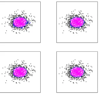
We now present two synthetic examples to illustrate this approach and its behavior. In both
examples, there are n=1000 points in the training set with D=2. The first example has 502 points
with label yi =−1 and 498 points with label yi = +1 and is separable by an elliptical decision
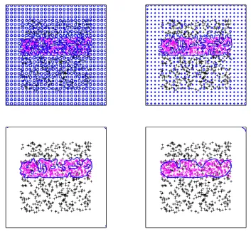
boundary. The second example has 400 points with label yi=−1 and 600 points with label yi= +1
and is not separable by a simple shape, but has the−1 labeled points in a strip.
In these two examples, in the other examples in the rest of the paper, and in the performance results of Section 5.2, we use the logistic loss function for L in the objective (7). In these two
examples, the surface area penalty has weightλ=0.5; the valueλ=0.5 is a default parameter value
that gives good performance with a variety of data sets regardless of their dimensionality D and can
be used if one does not wish to optimizeλusing cross-validation. Contour evolution minimization
requires an initial decision boundary. In the portion of Ωwhere there are no training examples,
we set the initial decision boundary to be a uniform grid of small components; this small seed
initialization is common in level set methods. In the part ofΩwhere there are training examples, we
Figure 3: Curve evolution iterations withλ=0.5 for an example training set proceeding in raster
scan order starting from the top left. The magenta×markers indicate class label−1 and
the black+markers indicate class label+1. The blue line is the decision boundary.
Two intermediate iterations and the final decision boundary are also shown in Figure 3 and Fig-ure 4. Solutions are as expected: an elliptical decision boundary and a strip-like decision boundary have been recovered. In the final decision boundaries of both examples, there is a small curved piece
of the decision boundary in the top right corner of Ωwhere there are no training examples. This
piece is an artifact of the initialization and the regularization term, and does not affect classifier performance. (The corner piece of the decision boundary is a minimal surface, a surface of zero mean curvature, which is a critical point of the surface area regularization functional (3), but not the global minimum. It is not important, assuming we have a representative training set.)
For a visual comparison of the effect of the surface area penalty weight, we show the solution
decision boundaries of the geometric level set classifier for two other values ofλ, 0.005 and 0.05,
with the data set used in the example of Figure 4. As can be seen in comparing this figure with the
bottom right panel of Figure 4, the smaller the value ofλ, the longer and more tortuous the decision
Figure 4: Curve evolution iterations withλ=0.5 for an example training set proceeding in raster
scan order starting from the top left. The magenta×markers indicate class label−1 and
the black+markers indicate class label+1. The blue line is the decision boundary.
In this section, we have described the basic method for nonlinear margin-based binary classi-fication based on level set methods and illustrated its operation on two synthetic data sets. The next two sections build upon this core binary level set classification in two directions: theoretical analysis, and multicategory classification.
3. Consistency and Complexity Analysis
In this section, we provide analytical characterizations of the consistency and complexity of the level set classifier with surface area regularization described in Section 2. The main tool used in these
characterizations isε-entropy. Once we have an expression for theε-entropy of the set of geometric
level set classifiers, we can then apply consistency and complexity results from learning theory that
are based on it. The beginning of this section is devoted to finding the ε-entropy of the space of
(a) (b)
Figure 5: Solution decision boundaries with (a)λ=0.005 and (b)λ=0.05 for an example training
set. The magenta×markers indicate class label−1 and the black +markers indicate
class label+1. The blue line is the decision boundary.
functions. The end of the section gives results on classifier consistency and complexity. The main findings are that level set classifiers are consistent, and that complexity is monotonically related to the surface area constraint, and thus the regularization term can be used to prevent underfitting and overfitting.
3.1 ε-Entropy
Theε-covering number of a metric space is the minimal number of sets with radius not exceeding
εrequired to cover that space. Theε-entropy is the base-two logarithm of the ε-covering number.
These quantities are useful values in characterizing learning (Kulkarni, 1989; Williamson et al., 2001; Lin, 2004; von Luxburg and Bousquet, 2004; Steinwart, 2005; Bartlett et al., 2006).
Kol-mogorov and Tihomirov (1961), Dudley (1974, 1979), and others provide ε-entropy calculations
for various classes of functions and various classes of sets, but the particular class we are consid-ering, signed distance functions with a constraint on the surface area of the zero level set, does not appear in the literature. The second and third examples in Section 2 of Kolmogorov and
Ti-homirov (1961) are related, and the general approach we take for obtaining theε-entropy of level
set classifiers is similar to those two examples.
In classification, it is always possible to scale and shift the data and this is often done in practice. Without losing much generality and dispensing with some bothersome bookkeeping, we consider
signed distance functions defined on the unit hypercube, that is Ω= [0,1]D, and we employ the
uniform or L∞metric,ρ∞(ϕ1,ϕ2) =supx∈Ω|ϕ1(x)−ϕ2(x)|. We denote the set of all signed distance
functions whose zero level set has surface area less than s by
F
s, itsε-covering number with respectto the uniform metric as Nρ∞,ε(
F
s), and itsε-entropy as Hρ∞,ε(F
s). We begin with the D=1 case and then come to general D.con-0 1 −1
0 1
x
ϕ
0 1
−1 0 1
x
ϕ
0 1
−1 0 1
x
ϕ
(a) (b) (c)
Figure 6: A D=1-dimensional signed distance function inΩ= [0,1]is shown in (a), marked with
its zero level set. Theε-corridor withε= 1
12 that contains the signed distance function
is shown in (b), shaded in gray. Theε-corridor of (b), whose center line has three zero
crossings is shown in (c), again shaded in gray, along with anε-corridor whose center
line has two zero crossings, shaded in green with stripes, and anε-corridor whose center
line has one zero crossing, shaded in red with dots.
straint, its slope is either+1 or−1 almost everywhere. The slope changes sign exactly once between
two consecutive points in the zero level set. The signed distance function takes values in the range
between positive and negative one.3 In the D=1 context, by surface area we mean the number of
points in the zero level set, for example three in Figure 6a.
In finding Hρ∞,ε(
F
s), we will use sets known asε-corridors, which are particular balls of radiusε measured usingρ∞ in the space of signed distance functions. We use the terminology of
Kol-mogorov and Tihomirov (or translator Hewitt), but our definition is slightly different than theirs. An ε-corridor is a strip of height 2εfor all x. Let us defineν=⌈ε−1⌉. At x=0, the bottom and top of a corridor are at 2 jεand 2(j+1)εrespectively for some integer j, where−ν≤2 j<ν. The slope
of the corridor is either+1 or −1 for all x and the slope can only change at values of x that are
multiples ofε. Additionally, the center line of theε-corridor is a signed distance function, changing
slope halfway between consecutive points in its zero level set and only there. The ε-corridor in
which the signed distance function of Figure 6a falls is indicated in Figure 6b. Otherε-corridors are
shown in Figure 6c.
By construction, each signed distance function is a member of exactly one ε-corridor. This is
because since at x=0 the bottom and top ofε-corridors are at consecutive integer multiples of 2ε
and since the center line of the corridor is a signed distance function, each signed distance function starts in oneε-corridor at x=0 and does not escape from it in the interval(0,1]. Also, anε-corridor whose center line has s points in its zero level set contains only signed distance functions with at least s points in their zero level sets.
3. There are several ways to define the signed distance function in the degenerate cases (R =Ω,Rc=/0) and (R =/0,
(Each piece has widthεexcept the last one ifε− is not an integer.) In each of theνsubintervals, the
center line of a corridor is either wholly positive or wholly negative. Enumerating the full set ofε
-corridors is equivalent to enumerating binary strings of lengthν. Thus, without a constraint s, there
are 2ν ε-corridors. Since, by construction, ε-corridors tile the space of signed distance functions,
Nρ∞,ε(
F
) =2ν.With the s constraint onε-corridors, the enumeration is equivalent to twice the number of
com-positions of the positive integerνby a sum of s or less positive integers. Twice because for every
composition, there is one version in which the first subinterval of the corridor center is positive and one version in which it is negative. As an example, the red corridor in Figure 6c can be composed
with two positive integers (5+7), the green corridor by three (7+4+1), and the gray corridor by
four (1+4+4+3). The number of compositions of νby k positive integers is νk−−11. Note that
the zero-crossings are unordered for this enumeration and that the set
F
sincludes all of the signeddistance functions with surface area smaller than s as well. Therefore:
Nρ∞,ε(
F
s) =2 s∑
k=1
ν −1 k−1
.
The result then follows because Hρ∞,ε(
F
s) =log2Nρ∞,ε(F
s).The combinatorial formula in Theorem 1 is difficult to work with, so we give a highly accurate approximation.
Theorem 2 Theε-entropy of the set of signed distance functions defined overΩ= [0,1]with zero level set having less than s points is:
Hρ∞,ε(
F
s)≈ε−1
+log2Φ 2s−
ε−1 p
⌈ε−1⌉ −1
! ,
whereΦis the standard Gaussian cumulative distribution function (cdf).
Proof Note that for a binomial random variable Z with (ν−1) Bernoulli trials having success probability 12:
Pr[Z<z] =2−ν·2 z
∑
k=1
ν −1 k−1
,
The central limit theorem tells us that the approximation works well when the Bernoulli suc-cess probability is one half, which it is in our case, and when the number of trials is large, which
corresponds to smallε. The continuous approximation is better in the middle of the domain, when
s≈ν/2, than in the tails. However, in the tails, the calculation of the exact expression in Theorem 1
is tractable. Since Φ is a cdf taking values in the range zero to one, log2Φ is nonpositive. The
surface area constraint only serves to reduce theε-entropy.
Theε-entropy calculation in Theorem 1 and Theorem 2 is for the D=1 case. We now discuss
the case with general D. Recall thatΩ= [0,1]D. Once again, we constructε-corridors that tile the space of signed distance functions. In the one-dimensional case, the ultimate object of interest for
enumeration is a string of lengthνwith binary labels. In the two-dimensional case, the
correspond-ing object is a ν-by-νgrid ofε-by-ε squares with binary labels, and in general a D-dimensional
Cartesian grid of hypercubes of volumeεD,νon each side. The surface area of the zero level set
is the number of interior faces in the Cartesian grid whose adjoiningεDhypercubes have different
binary labels.
Theorem 3 Theε-entropy of the set of signed distance functions defined overΩ= [0,1]Dwith zero level set having surface area less than s is:
Hρ∞,ε(
F
s)≈ε−1D
+log2Φ
2s−D ε−1−1 ε−1D−1−1
q
D(⌈ε−1⌉ −1)⌈ε−1⌉D−1
,
whereΦis the standard Gaussian cdf.
Proof In the one-dimensional case, it is easy to see that the number of segments isνand the number
of interior faces isν−1. For a general D-dimensional Cartesian grid withνhypercubes on each
side, the number of hypercubes isνDand the number of interior faces is D(ν−1)νD−1. The result follows by substitutingνDforνand D(ν−1)νD−1forν−1 in Theorem 2.
Theorem 2 is a special case of Theorem 3 with D=1. It is common to find the dimension of
the space D in the exponent ofε−1inε-entropy calculations as we do here.
Theε-entropy calculation for level set classifiers given here enables us to analytically
character-ize their consistency properties as the scharacter-ize of the training set goes to infinity in Section 3.2 through
ε-entropy-based classifier consistency results. The calculation also enables us to characterize the
Rademacher complexity of level set classifiers in Section 3.3 throughε-entropy-based complexity
results.
3.2 Consistency
In the binary classification problem, with training set of size n drawn from pX,Y(x,y), a consistent classifier is one whose probability of error converges in the limit as n goes to infinity to the probabil-ity of error of the Bayes optimal decision rule. The optimal decision rule to minimize the probabilprobabil-ity of error is ˆy∗(x) =sign(pY|X(Y =1|X=x)−12). Introducing notation, let the probability of error
achieved by this decision rule be R∗. Also denote the probability of error of a level set classifier
also be analyzed; since the regularization term based on surface area we introduce is new, so is the following analysis.
Concentrating on the surface area regularization, we adapt Theorem 4.1 of Lin, which is based
on ε-entropy. The analysis is based on the method of sieves, where sieves
F
n are an increasingsequence of subspaces of a function space
F
. In our case,F
is the set of signed distance functionson Ω and the sieves,
F
s(n), are subsets of signed distance functions whose zero level sets havesurface area less than s(n), that isH
ϕ=0ds<s(n). Such a constraint is related to the regularization
expression E(ϕ)given in (7) through the method of Lagrange multipliers, withλinversely related
to s(n). In the following, the function s(n)is increasing in n and thus the conclusions of the theorem provide asymptotic results on consistency as the strength of the regularization term decreases as more training samples are made available. The sieve estimate is:
ϕ(n)=arg min ϕ∈Fs(n)
n
∑
i=1
L(yiϕ(xi)). (9)
Having found Hρ∞,ε(
F
s) in Section 3.1, we can apply Theorem 4.1 of Lin (2004), yielding thefollowing theorem.
Theorem 4 Let L be a Fisher-consistent loss function in (9); let ˜ϕ=arg minϕ∈FE[L(Yϕ(X))],
where
F
is the space of signed distance functions on[0,1]D; and letF
s(n)be a sequence of sieves. Then for sieve estimateϕ(n), we have4
R(sign(ϕ(n)))−R∗=O P
max
n−τ, inf
ϕ∈Fs(n)
Z
(ϕ(x)−ϕ˜(x))2pX(x)dx
,
where
τ=
1
3, D=1
1 4−
log log n
2 log n , D=2 1
2D, D≥3
.
Proof The result is a direct application of Theorem 4.1 of Lin (2004), which is in turn an
appli-cation of Theorem 1 of Shen and Wong (1994). In order to apply this theorem, we need to note
two things. First, that signed distance functions on[0,1]Dare bounded (by a value of 1) in the L
∞
norm. Second, that there exists an A such that Hρ∞,ε(
F
s)≤Aε−D. Based on Theorem 3, we seethat Hρ∞,ε(
F
s)≤νDbecause the logarithm of the cdf is nonpositive. Sinceν=⌈ε−1⌉, ifε−1 is an integer, then Hρ∞,ε(F
s)≤ε−Dand otherwise there exists an A such that Hρ∞,ε(F
s)≤Aε−D.Clearly n−τgoes to zero as n goes to infinity. Also, infϕ∈Fs(n)R(ϕ(x)−ϕ˜(x))2pX(x)dx goes to
zero when s(n)is large enough so that the surface area constraint is no longer applicable.5 Thus,
level set classifiers are consistent.
3.3 Rademacher Complexity
The principal idea of the structural risk minimization principle is that the generalization error is the sum of an empirical risk term and a capacity term (Vapnik, 1995). The two terms should be
sensibly balanced in order to achieve low generalization error. Here, we use theε-entropy of signed
distance functions constrained in decision boundary surface area to characterize the capacity term.
In particular, we look at the Rademacher complexity of
F
sas a function of s (Koltchinskii, 2001;Bartlett and Mendelson, 2002).
The Rademacher average of a class
F
, denoted ˆRn(F
), satisfies (von Luxburg and Bousquet,2004):
ˆ
Rn(
F
)≤2ε+ 4√2√
n
Z ∞
ε
4 q
Hρ2,n,ε′(
F
)dε′,whereρ2,n(ϕ1,ϕ2) =
q
1 n∑
n
i=1(ϕ1(xi)−ϕ2(xi))2is the empiricalℓ2metric. We found Hρ∞,ε(
F
s)for signed distance functions with surface area less than s in Section 3.1, and Hρ2,n,ε(F
)≤Hρ∞,ε(F
).Thus, we can characterize the complexity of level set classifiers via the Rademacher capacity term (von Luxburg and Bousquet, 2004):
CRad(
F
s,n) =2ε+ 4√2√n
Z ∞
ε
4 q
Hρ∞,ε′(
F
)dε′. (10)WithΩ= [0,1]D, the upper limit of the integral in (10) is one rather than infinity becauseεcannot be greater than one.
In Figure 7, we plot CRad as a function of s for three values of D, and fixedεand n. Having a
fixedεmodels the discretized grid implementation of level set methods. As the value of s increases,
decision boundaries with more area are available. Decision boundaries with large surface area are more complex than smoother decision boundaries with small surface area. Hence the complexity term increases as a function of s. We have also empirically found the same relationship between the VC dimension and the surface area penalty (Varshney and Willsky, 2008). Consequently, the surface area penalty can be used to control the complexity of the classifier, and prevent underfitting and overfitting. The Rademacher capacity term may be used in setting the regularization parameter λ.
4. Multicategory Geometric Level Set Classification
Thus far, we have considered binary classification. In this section, we extend level set classification
to the multicategory case with M>2 classes labeled y∈ {1, . . . ,M}. We represent the decision
boundaries using m=⌈log2M⌉ signed distance functions {ϕ1(x), . . . ,ϕm(x)}. Using such a set of level set functions we can represent 2m regions {
R
1,R
2, . . . ,R
2m} through a binary encodingx 10 x 10
(a) (b) (c)
Figure 7: The Rademacher capacity term (10) as a function of s for signed distance functions on
Ω= [0,1]Dwith surface area less than s with (a) D=2, (b) D=3, and (c) D=4. The
values ofεand n are fixed at 0.01 and 1000 respectively.
(Vese and Chan, 2002). Thus, for x∈
R
1,(ϕ1(x)<0)∧ ··· ∧(ϕm(x)<0); for x∈R
2,(ϕ1(x)< 0)∧ ··· ∧(ϕm−1(x)<0)∧(ϕm>0); and for x∈R
2m,(ϕ1(x)>0)∧ ··· ∧(ϕm(x)>0).This binary encoding specifies the regions, but in order to apply margin-based loss functions,
we also need a value for margin. In binary classification, the special encoding y∈ {−1,+1}
al-lows yϕ(x) to be the argument to the loss function. For multicategory classification, the
argu-ment to the loss function is through functionsψy(x), which are also specified through a binary
en-coding: ψ1(x) =max{+ϕ1(x), . . . ,+ϕm(x)},ψ2(x) =max{+ϕ1(x), . . . ,+ϕm−1(x),−ϕm(x)}, and
ψ2m(x) =max{−ϕ1(x), . . . ,−ϕm(x)}. Then, the M-ary level set classification energy functional we
propose is
E(ϕ1, . . . ,ϕm) = n
∑
i=1
L(ψyi(xi)) +
λ m
m
∑
j=1
I
ϕj=0
ds. (11)
The same margin-based loss functions used in the binary case, such as the hinge and logistic loss functions, may be used in the multicategory case (Zou et al., 2006, 2008). The regularization term included in (11) is the sum of the surface areas of the zero level sets of the m signed distance functions.
The gradient descent flows for the m signed distance functions are
∂ϕ1(x) ∂t
x=xi
= (
L(ψyi(xi))∇ϕ1(xi)−
λ
m∇2ϕ1(xi)∇ϕ1(xi), ϕ1(xi)<0
−L(ψyi(xi))∇ϕ1(xi)−mλ∇
2ϕ
1(xi)∇ϕ1(xi), ϕ1(xi)>0 ..
. ∂ϕm(x)
∂t
x=xi
= (
L(ψyi(xi))∇ϕm(xi)−
λ
m∇ 2ϕ
m(xi)∇ϕm(xi), ϕm(xi)<0
−L(ψyi(xi))∇ϕm(xi)−
λ
m∇2ϕm(xi)∇ϕm(xi), ϕm(xi)>0
.
In the case M=2 and m=1, the energy functional and gradient flow revert back to binary level set
classification described in Section 2.
both because it treats all M classes simultaneously in the objective and because the decision regions are represented by a logarithmic rather than linear number of decision functions. Zou et al. (2006) also treat all M classes simultaneously in the objective, but their multicategory kernel machines use M decision functions. In fact, to the best of our knowledge, there is no M-ary classifier
represen-tation in the literature using as few as⌈log2M⌉decision functions. Methods that combine binary
classifier outputs using error-correcting codes make use of a logarithmic number of binary
classi-fiers with a larger multiplicative constant, such as ⌈10 log M⌉or ⌈15 log M⌉ (Rifkin and Klautau,
2004; Allwein et al., 2000).
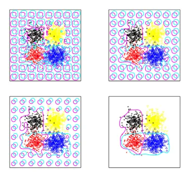
We give an example showing multicategory level set classification with M=4 and D=2. The
data set has 250 points for each of the four class labels yi =1, yi =2, yi=3, and yi =4. The
classes are not perfectly separable by simple boundaries. With four classes, we use m=2 signed
distance functions. Figure 8 shows the evolution of the two contours, the magenta and cyan curves.
The final decision region for class y=1 is the portion inside both the magenta and cyan curves,
and coincides with the training examples with class label 1. The final decision region for class 2 is the region inside the magenta curve but outside the cyan curve, the final decision region for class 3 is the region inside the cyan curve, but outside the magenta curve, and the final decision region for class 4 is outside both curves. The final decision boundaries are fairly smooth and partition the space with small training error.
5. Implementation and Classification Results
In this section, we describe how to implement geometric level set classification practically using RBFs and give classification performance results when applied to several real binary and multicat-egory data sets.
5.1 Radial Basis Function Level Set Method
There have been many developments in level set methods since the original work of Osher and Sethian (1988). One development in particular is to represent the level set function by a superposi-tion of RBFs instead of on a grid (Cecil et al., 2004; Slabaugh et al., 2007; Gelas et al., 2007). Grid-based representation of the level set function is not amenable to classification in high-dimensional input spaces because the memory and computational requirements are exponential in the dimension of the input space. A nonparametric RBF representation, however, is tractable for classification. The RBF level set method we use to minimize the energy functionals (7) and (11) for binary and multicategory margin-based classification is most similar to that described by Gelas et al. (2007) for image processing.
The starting point of the RBF level set approach is describing the level set functionϕ(x)via a
strictly positive definite6RBF K(·)as follows: ϕ(x) =
n
∑
i=1
αiK(kx−xik). (12)
The zero level set ofϕdefined in this way is the contour C. For the classification problem, we take
the centers xi to be the data vectors of the training set. Then, constructing an n×n matrix H with
Figure 8: Curve evolution iterations with λ=0.5 for multicategory classification proceeding in
raster scan order. The red×markers indicate class label 1, the black+markers indicate
class label 2, the blue△markers indicate class label 3, and the yellow▽markers indicate
class label 4. The magenta and cyan lines are the zero level sets of the m=2 signed
elements{H}i j=K(kxi−xjk), and lettingαααbe the vector of coefficients in (12), we have:
ϕ(x1) .. . ϕ(xn)
=Hααα.
To minimize an energy functional of C, the level set optimization is over the coefficientsαααwith
H fixed. In order to perform contour evolution with the RBF representation, a time parameter t is
introduced like in Section 2, giving:
Hdααα
dt =
∂ϕ(x) ∂t
x=x1 .. .
∂ϕ(x) ∂t
x=xn
. (13)
For the binary margin-based classification problem with surface area regularization that we are inter-ested in solving, we substitute the gradient flow (8) into the right side of (13). For the multicategory classification problem, we have m level set functions as discussed in Section 4 and each one has a gradient flow to be substituted into an expression like (13).
The iteration for the contour evolution is then:
ααα(k+1)=ααα(k)
−τH−1
∂ϕ(k)(x) ∂t
x=x1 .. .
∂ϕ(k)(x) ∂t
x=xn
, (14)
whereτis a small step size andϕ(k) comes fromααα(k). We normalizeαααaccording to theℓ1-norm after every iteration.
The RBF-represented level set function is not a signed distance function. However, as discussed by Gelas et al. (2007), normalizing the coefficient vectorαααwith respect to theℓ1-norm after every it-eration of (14) has a similar effect as reinitializing the level set function as a signed distance function. The Lipschitz constant of the level set function is constrained by this normalization. The analysis of Section 3 applies with minor modification for level set functions with a given Lipschitz constant and surface area constraint. The RBF level set approach is similar to kernel machines with the RBF kernel in the sense that the decision function is represented by a linear combination of RBFs. How-ever, kernel methods in the literature minimize a reproducing kernel Hilbert space squared norm for regularization, whereas the geometric level set classifier minimizes decision boundary surface area for regularization. The regularization term and consequently inductive bias of the geometric level set classifier is new and different compared to existing kernel methods. The solution decision boundary is the zero level set of a function of the form given in (12). Of course this representation does not capture all possible functions, but, given that we use a number of RBFs equal to the num-ber of training examples, the granularity of this representation is well-matched to the data. This is similar to the situation found in other contexts such as kernel machines using RBFs.
Figure 9: Curve evolution iterations with RBF implementation andλ=0.5 for example training set
proceeding in raster scan order. The magenta×markers indicate class label−1 and the
black+markers indicate class label+1. The blue line is the decision boundary.
contour evolution on the elliptically-separable data set presented in Section 2. The initial decision boundary is tortuous. It is smoothed out by the surface area penalty during the course of the contour evolution, thereby improving the generalization of the learned classifier as desired. To initialize the m vectorsαααin M category classification, we use m length n vectors of positive and negative ones constructed from the binary encoding instead of y.
5.2 Classification Results
We give classifier performance results on benchmark data sets from the UCI Machine Learning Repository (Asuncion and Newman, 2007) for geometric level set classification and compare them to the performance of several other classifiers, concluding that level set classification is a compet-itive technique. We present the tenfold cross-validation classification error performance with RBF
Wis-0.1 0.2 0.4 0.8 1.6 3.2 6.4 0
0.05 0.1 0.15 0.2 0.25 0.3
classification error
λ 0.1 0.2 0.4 0.8 1.6 3.2 6.4
0 0.02 0.04 0.06 0.08
classification error
λ
(a) (b)
Figure 10: Tenfold cross-validation training error (blue line with triangle markers) and test error (red line with circle markers) for the (a) Pima, and (b) WDBC data sets as a function of
the regularization parameterλon a logarithmic scale.
consin Diagnostic Breast Cancer (n=569, D=30), BUPA Liver Disorders (n=345, D=6) and
Johns Hopkins University Ionosphere (n=351, D=34), and four multicategory data sets: Wine
Recognition (n=178, M=3, D=13), Iris (n=150, M=3, D=4), Glass Identification (n=214,
M=6, D=9), and Image Segmentation (n=2310, M=7, D=19). For the binary data sets, there
is m=1 level set function, for the wine and iris data sets m=2 level set functions, and for the glass
and segmentation data sets m=3 level set functions.
We shift and scale the data so that each of the input dimensions has zero mean and unit variance, use the RBF K(kx−xik) =e−kx−xik
2
, the logistic loss function, τ=1/m, and the initialization
ααα=n(H−1y)/kH−1yk1. First, we look at classification error as a function ofλ. Figure 10 shows the tenfold cross-validation training and test errors for the Pima and WDBC data sets; other data sets yield similar plots. The plots show evidence of the structural risk minimization principle and
complexity analysis given in Section 3.3. For smallλ(corresponding to large surface area constraint
s), the model class is too complex and we see that although the training error is zero, the test error
is not minimal due to overfitting. For largeλ, the model class is not complex enough; the training
error is large and the test error is not minimal due to underfitting. There is an intermediate value of
λthat achieves the minimal test error. However, we notice that the test error is fairly insensitive to
the value ofλ. The test error does not change much over the plotted range.
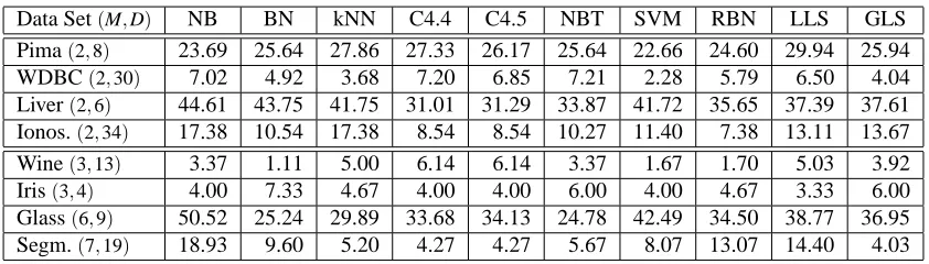
In Table 1, we report the tenfold cross-validation test error (as a percentage) on the eight data
sets and compare the performance to nine other classifiers.7 On each of the ten folds, we setλusing
cross-validation. Specifically, we perform fivefold cross-validation on the nine tenths of the full data set that is the training data for that fold. We select theλfrom the set of values{0.2,0.4,0.8,1.6,3.2} that minimizes the fivefold cross-validation test error. The performance results of the nine other
Segm.(7,19) 18.93 9.60 5.20 4.27 4.27 5.67 8.07 13.07 14.40 4.03
Table 1: Tenfold cross-validation error percentage of geometric level set classifier (GLS) with RBF level set implementation on several data sets compared to error percentages of various other classifiers reported in Cai and Sowmya (2007). The other classifiers are: na¨ıve Bayes classifier (NB), Bayes net classifier (BN), k-nearest neighbor with inverse distance weight-ing (kNN), C4.4 decision tree (C4.4), C4.5 decision tree (C4.5), na¨ıve Bayes tree classifier (NBT), SVM with polynomial kernel (SVM), radial basis function network (RBN), and learning level set classifier (LLS) of Cai and Sowmya (2007).
classifiers are as given by Cai and Sowmya (2007), who report the same tenfold cross-validation test error that we do for the geometric level set classifier. Details about parameter settings for the other nine classifiers may be found in Cai and Sowmya (2007).
The geometric level set classifier outperforms each of the other classifiers at least once among the four binary data sets, and is generally competitive overall. Level set classification is also com-petitive on the multicategory data sets. In fact, it gives the smallest error among all of the classifiers on the segmentation data set. The proposed classifier is competitive for data sets of both small and large dimensionality D; there is no apparent relationship between D and the performance of the geometric level set classifier in comparison to other methods.
6. Conclusion
Level set methods are powerful computational techniques that have not yet been widely adopted in machine learning. Our main goal with this contribution is to open a conduit between the appli-cation area of learning and the computational technique of level set methods. Towards that end, we have developed a nonlinear, nonparametric classifier based on level set methods that minimizes margin-based empirical risk in both the binary and multicategory cases, and is regularized by a geo-metric complexity penalty novel to classification. This approach is an alternative to kernel machines for learning nonlinear decision boundaries in the input space and is in some ways a more natural generalization of linear methods.
The variational level set formulation is flexible in allowing the inclusion of various geometric priors defined in the input space. The surface area regularization term is one such example, but oth-ers may also be included. Another example is an energy functional that measures feature relevance using the partial derivative of the signed distance function (Domeniconi et al., 2005), and can be
We have provided an analysis of the classifier by characterizing itsε-entropy. This characteri-zation leads to results on consistency and complexity. We have described a multicategory level set classification procedure with a logarithmic number of decision functions, rather than the linear num-ber that is typical in classification and decision making, through a binary encoding made possible by the level set representation.
It is a known fact that with finite training data, no one classification method is best for all data sets. Performance of classifiers may vary quite a bit depending on the data characteristics because of differing inductive biases. The classifier presented in this paper provides a new option when choosing a classifier. The results on standard data sets indicate that the level set classifier is com-petitive with other state-of-the-art classifiers. It would be interesting to systematically find domains in the space of data set characteristics for which the geometric level set classifier outperforms other classifiers (Ho and Basu, 2002).
Acknowledgments
This work was supported in part by an NSF Graduate Research Fellowship, by Shell International Exploration and Production, Inc., and by a MURI funded through ARO Grant W911NF-06-1-0076. The authors thank Justin H. G. Dauwels, John W. Fisher, III and Sujay R. Sanghavi for discussions. The level set methods toolbox by Barıs¸ S¨umengen was used in producing figures in Section 2 and Section 4.
References
Shotaro Akaho. SVM that maximizes the margin in the input space. Systems and Computers in Japan, 35(14):78–86, December 2004.
Erin L. Allwein, Robert E. Schapire, and Yoram Singer. Reducing multiclass to binary: A unifying approach to margin classifiers. Journal of Machine Learning Research, 1:113–141, December 2000.
Arthur Asuncion and David J. Newman. UCI machine learning repository. Available at
http://archive.ics.uci.edu/ml/, 2007.
Peter L. Bartlett and Shahar Mendelson. Rademacher and Gaussian complexities: Risk bounds and structural results. Journal of Machine Learning Research, 3:463–482, November 2002.
Peter L. Bartlett, Michael I. Jordan, and Jon D. McAuliffe. Convexity, classification, and risk bounds. Journal of the American Statistical Association, 101(473):138–156, March 2006.
Gilles Blanchard, Christin Sch¨afer, Yves Rozenholc, and Klaus-Robert M¨uller. Optimal dyadic decision trees. Machine Learning, 66(2–3):209–241, March 2007.
Thomas Cecil, Jianliang Qian, and Stanley Osher. Numerical methods for high dimensional Hamilton–Jacobi equations using radial basis functions. Journal of Computational Physics, 196 (1):327–347, May 2004.
Daniel Cremers, Mikael Rousson, and Rachid Deriche. A review of statistical approaches to level set segmentation: Integrating color, texture, motion and shape. International Journal of Computer Vision, 72(2):195–215, April 2007.
Michel C. Delfour and Jean-Paul Zol´esio. Shapes and Geometries: Analysis, Differential Calculus, and Optimization. Society for Industrial and Applied Mathematics, Philadelphia, Pennsylvania, 2001.
Carlotta Domeniconi, Dimitrios Gunopulos, and Jing Peng. Large margin nearest neighbor classi-fiers. IEEE Transactions on Neural Networks, 16(4):899–909, July 2005.
Richard M. Dudley. Metric entropy of some classes of sets with differentiable boundaries. Journal of Approximation Theory, 10(3):227–236, March 1974.
Richard M. Dudley. Correction to “metric entropy of some classes of sets with differentiable bound-aries”. Journal of Approximation Theory, 26(2):192–193, June 1979.
Bradley Efron. The efficiency of logistic regression compared to normal discriminant analysis. Journal of the American Statistical Association, 70(352):892–898, December 1975.
Arnaud Gelas, Olivier Bernard, Denis Friboulet, and R´emy Prost. Compactly supported radial basis functions based collocation method for level-set evolution in image segmentation. IEEE Transactions on Image Processing, 16(7):1873–1887, July 2007.
Tin Kam Ho and Mitra Basu. Complexity measures of supervised classification problems. IEEE Transactions on Pattern Analysis and Machine Intelligence, 24(3):289–300, March 2002.
Chih-Wei Hsu and Chih-Jen Lin. A comparison of methods for multiclass support vector machines. IEEE Transactions on Neural Networks, 13(2):415–425, March 2002.
Andrey N. Kolmogorov and Vladimir M. Tihomirov. ε-entropy andε-capacity of sets in functional
spaces. American Mathematical Society Translations Series 2, 17:277–364, 1961.
Vladimir Koltchinskii. Rademacher penalties and structural risk minimization. IEEE Transactions on Information Theory, 47(5):1902–1914, July 2001.
Yi Lin. A note on margin-based loss functions in classification. Statistics & Probability Letters, 68 (1):73–82, June 2004.
Ulrike von Luxburg and Olivier Bousquet. Distance-based classification with Lipschitz functions. Journal of Machine Learning Research, 5:669–695, June 2004.
Stanley Osher and Ronald Fedkiw. Level Set Methods and Dynamic Implicit Surfaces. Springer, New York, 2003.
Stanley Osher and James A. Sethian. Fronts propagating with curvature-dependent speed: Algo-rithms based on Hamilton–Jacobi formulations. Journal of Computational Physics, 79(1):12–49, November 1988.
Nikos Paragios and Rachid Deriche. Geodesic active regions and level set methods for supervised texture segmentation. International Journal of Computer Vision, 46(3):223–247, February 2002.
Georg P¨olzlbauer, Thomas Lidy, and Andreas Rauber. Decision manifolds—a supervised learning algorithm based on self-organization. IEEE Transactions on Neural Networks, 19(9):1518–1530, September 2008.
Ryan Rifkin and Aldebaro Klautau. In defense of one-vs-all classification. Journal of Machine Learning Research, 5:101–141, January 2004.
Frank Rosenblatt. The perceptron: A probabilistic model for information storage and organization in the brain. Psychological Review, 65(6):386–408, 1958.
Christophe Samson, Laure Blanc-F´eraud, Gilles Aubert, and Josiane Zerubia. A level set model for image classification. International Journal of Computer Vision, 40(3):187–197, December 2000.
Bernhard Sch¨olkopf and Alexander J. Smola. Learning with Kernels: Support Vector Machines, Regularization, Optimization, and Beyond. MIT Press, Cambridge, Massachusetts, 2002.
Clayton Scott and Robert D. Nowak. Minimax-optimal classification with dyadic decision trees. IEEE Transactions on Information Theory, 52(4):1335–1353, April 2006.
Xiaotong Shen and Wing Hung Wong. Convergence rate of sieve estimates. The Annals of Statistics, 22(2):580–615, June 1994.
Jianbo Shi and Jitendra Malik. Normalized cuts and image segmentation. IEEE Transactions on Pattern Analysis and Machine Intelligence, 22(8):888–905, August 2000.
Gregory G. Slabaugh, H. Quynh Dinh, and G¨ozde B. Unal. A variational approach to the evolution of radial basis functions for image segmentation. In Proceedings of the IEEE Computer Society Conference on Computer Vision and Pattern Recognition, Minneapolis, Minnesota, June 2007.
Ingo Steinwart. Consistency of support vector machines and other regularized kernel classifiers. IEEE Transactions on Information Theory, 51(1):128–142, January 2005.
Systems, pages 303–310, Rydzyna, Poland, 2005.
Arkadiusz Tomczyk and Piotr S. Szczepaniak. Adaptive potential active hypercontours. In Leszek Rutkowski, Ryszard Tadeusiewicz, Lotfi A. Zadeh, and Jacek Zurada, editors, Proceedings of the 8th International Conference on Artificial Intelligence and Soft Computing, pages 692–701, Zakopane, Poland, June 2006.
Arkadiusz Tomczyk, Piotr S. Szczepaniak, and Michal Pryczek. Active contours as knowledge discovery methods. In Vincent Corruble, Masayuki Takeda, and Einoshin Suzuki, editors, Pro-ceedings of the 10th International Conference on Discovery Science, pages 209–218, Sendai, Japan, 2007.
Aad W. van der Vaart. Asymptotic Statistics. Cambridge University Press, Cambridge, England, 1998.
Vladimir N. Vapnik. The Nature of Statistical Learning Theory. Springer, New York, 1995.
Kush R. Varshney and Alan S. Willsky. Supervised learning of classifiers via level set segmentation. In Proceedings of the IEEE Workshop on Machine Learning for Signal Processing, pages 115– 120, Canc´un, Mexico, October 2008.
Luminita A. Vese and Tony F. Chan. A multiphase level set framework for image segmentation using the Mumford and Shah model. International Journal of Computer Vision, 50(3):271–293, December 2002.
Holger Wendland. Scattered Data Approximation. Cambridge University Press, Cambridge, Eng-land, 2005.
Rebecca Willett and Robert D. Nowak. Minimax optimal level-set estimation. IEEE Transactions on Image Processing, 16(12):2965–2979, December 2007.
Robert C. Williamson, Alexander J. Smola, and Bernhard Sch¨olkopf. Generalization performance of regularization networks and support vector machines via entropy numbers of compact operators. IEEE Transactions on Information Theory, 47(6):2516–2532, September 2001.
Andy M. Yip, Chris Ding, and Tony F. Chan. Dynamic cluster formation using level set methods. IEEE Transactions on Pattern Analysis and Machine Intelligence, 28(6):877–889, June 2006.
Hui Zou, Ji Zhu, and Trevor Hastie. The margin vector, admissible loss and multi-class margin-based classifiers. Technical report, University of Minnesota, 2006.


![Figure 6: A D = 1-dimensional signed distance function in Ω = [0,1] is shown in (a), marked withits zero level set](https://thumb-us.123doks.com/thumbv2/123dok_us/9824418.1968393/11.612.105.512.89.215/figure-dimensional-signed-distance-function-shown-marked-withits.webp)
![Figure 7: The Rademacher capacity term (10) as a function of s for signed distance functions onΩ = [0,1]D with surface area less than s with (a) D = 2, (b) D = 3, and (c) D = 4](https://thumb-us.123doks.com/thumbv2/123dok_us/9824418.1968393/16.612.96.515.90.214/figure-rademacher-capacity-function-signed-distance-functions-surface.webp)