Water Quality Model for Streams: A Review

https://www.scirp.org/journal/jep ISSN Online: 2152-2219

ISSN Print: 2152-2197

DOI: 10.4236/jep.2019.1012097 Dec. 20, 2019 1612 Journal of Environmental Protection

Water Quality Model for Streams: A Review

S. Ranjith1 _{, Anand V. Shivapur}2_{, P. Shiva Keshava Kumar}3_, Chandrashekarayya G. Hiremath4_{, Santhosh Dhungana}5

1_{VTU-PG Studies, Belagavi, India}

2_{Department of Civil Engineering, VTU-PG Studies, Belagavi, India}

3_{Department of Civil Engineering, PDIT Engineering College, Hosapete, India} 4_{Department of Water and Land Management, VTU, Belagavi, India}

5_{School of Environment, Resources and Development (SERD), Pathumthani, Thailand}

Abstract

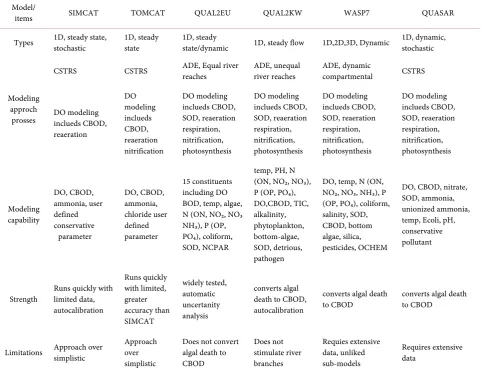
Six main public domain water quality models which are presently available for Rivers and streams are being captured in this article. These main models could produce important results if they are used in the correct manner, be-cause they are different in terms of assumptions, strength and weaknesses, processes they represent, modeling capability and data input requirements. The Model review discussed includes, water quality analysis simulation pro-gram (WASP7), simulation catchment (SIMCAT), quality simulation along Rivers (QUASAR), and the temporal overall model for catchment (TOMCAT), QUAL2KW, QUAL2EU. The models are described individually according to a consistent set of criteria-conceptualization, model capability, model strengths, limitations, input data and how it utilized. The outcome showed that TOMCAT and SIMCAT are important in ASSESSING effect of point sources in a very simple way. The QUAL2KW, unlike the QUAL2EU where macrophytes play a major interaction, it can convert algal death to carbonaceous Biochemical Oxygen Demand (CBOD), thereby making it more suitable. In addition to the extensive requirement of data, it is expensive and time consuming to set up these complex models such as QUASAR and WASP7. Therefore, one model cannot be used for all the required functional-ities. Choosing a model would depend on a specific application, financial cost and time availability. This article may be of help in choosing a suitable model for a specific water quality problem.

Keywords

Water Quality Models, Dissolved Oxygen, SIMCAT, TOMCAT, QUAL2Kw, QUAL2EU, WASP7 and QUASAR

How to cite this paper: Ranjith, S., Shivapur, A.V., Kumar, P.S.K., Hiremath, C.G. and Dhungana, S. (2019) Water Quality Model for Streams: A Review. Journal of Environ-mental Protection, 10, 1612-1648.

https://doi.org/10.4236/jep.2019.1012097

Received: August 7, 2019 Accepted: December 17, 2019 Published: December 20, 2019

Copyright © 2019 by author(s) and Scientific Research Publishing Inc. This work is licensed under the Creative Commons Attribution International License (CC BY 4.0).

http://creativecommons.org/licenses/by/4.0/

DOI: 10.4236/jep.2019.1012097 1613 Journal of Environmental Protection

1. Introduction

There are various ways of describing the mathematical model. A model de-scribed by the encyclopedia of life support system portrays it as an approximate description of a class of real-world objects and phenomena expressed by ma-thematical symbolisms [1]. The model was described by Concise Oxford dictio-nary (1990) as a simplified form of a system which aids calculations and predicts the Conditions of a system in a particular situation. Water quality models were described by US-EPA [2] as tools for simulating movement of pollutants and precipitation from the ground surface via pipe and network channels, storage treatment units and finally to receiving waters. Chapra [3] explained a mathe-matical model as an idealized formulation which shows the response of a physi-cal system from external stimuli. Similarly, a water quality model was described by Cox [4] as anything derived from a simple empirical relationship, via a set of mass balance equations, to a complex software suite by which water quality in streams and rivers can be simulated by a user, by providing chemical and physi-cal data.

An essential material required for the survival of aquatic life is Dissolved oxy-gen (DO). Reduced concentration of dissolved oxyoxy-gen leads to an imbalance in the ecosystem with odors, aesthetic nuisances and fish mortality [4]. A strategy for water quality management, involving the assessment of pollutant effects on the dissolved oxygen concentration along the river systems can be used to attain a particular water quality. In 1925, quantitative methods were used to assess the effects of pollutants on the river systems, when Phelps and Streeter created a model for the simulation of DO in the river systems.

Following the advancement in computer technology in the 20th _{and 21}st centu-ries, there has been numerous development in the aspect of water quality modelling which has brought about different models. Due to continuous stu-dies and construction of new models for particular events around the globe, there is now a variety of water quality models [4]. A compromise between de-sirability and feasibility should be considered in selecting a simulation model

[5]. Six most common and freely accessible water quality models have been addressed in this article, they include; QUAL2KW; QUAL2EU; Simulation catchment SIMCAT; water quality analysis program, WASP7; quality simulation along Rivers, QUASAR; and temporal overall model for catchments, TOMCAT, which are used for simulating dissolved oxygen along river systems and assessed each their potential for use in applications.

2. Model Review

DOI:10.4236/jep.2019.1012097 1614 Journal of Environmental Protection 2.1. SIMCAT

The SIMCAT is seen as a stochastic, one dimensional (1D), Steady state and de-terministic model. Anglian Water [6], a leading provider of water and wastewa-ter services in the United Kingdom (UK), developed SIMCAT. For over 20 years, it has been used commonly in the UK, and is known to be a not expensive, prac-tical tool for management of water quality. The quality of the river water has been described by this toll, throughout a catchment, using the Monte Carlo si-mulation technique, like mean and range of percentiles [7]. A well detailed ar-ticle on SIMCAT can be seen at Cox [4].

2.1.1. Conceptualization

According to SIMCAT, the stream system can be divided into diverse user well-defined spreads into any distance, which is occupied as the distance be-tween branches or supplementary points of interest. This model can perform greater than one influence in a particular reach. A diffuser run off can be classi-fied as quality and flow rate. The model depicts the river reaches as a continually stirred tank reactors in series (CSTRS) model. This model doesn’t utilize and advection-dispersion transport equation, but simulated instantaneous and per-fect mixing along the reach, with the movement of water and solutes at the same velocity. At the beginning of every reaching, a mass balance is performed. The solute mass-balances and the flow for a specific reach include;

0 i t c a

Q =Q +Q +Q −Q (1) And

0 0 i i t t e e i a

C Q =C Q +C Q +C Q −c Q ± ∆C (2) where Q = flow and C = concentration of determinants o, i, t, e = reach flow, upstream input, tributary inputs, effluents discharges, and abstractions, respec-tively. Physical, biological, or chemical processes are internal transformations which are depicted by the term ΔC. An empirical velocity–flow relationship (V = aQb, where V is the velocity, Q is the flow rate and a, b are constants) is used to get the water velocity in a particular reach. The residence time can be derived from the calculated velocity.

2.1.2. Processes

In order to calculate the concentration of determinants that will move to the next reach, the concentrations of the solute pass through first-order decays. The determinants which are being modeled might be treated as having first-order decay or conservatively, these models include; ammonium (first order), Bio-chemical oxygen demand (BOD first order), chloride (conservative). SIMCAT describes advective transport and chemical fate as

0

d d

, d and

d x

c x x

kc t C C e k

t = − = v = ⋅ − ⋅v (3)

DOI: 10.4236/jep.2019.1012097 1615 Journal of Environmental Protection included and the method of Elmore and Hayes [8] is used to estimate the DO saturation concentration as expressed by the equations,

(

)

d

d r a s

c

k L k c c

t = − + − (4)

2 3

14652 0.41022 0.0079910 0.000077774

s

c = − T+ T − T (5)

where C is the DO concentration, Cs is the saturation concentration, L is the BOD, kr is the rate of removal of BOD, ka is the re-aeration rate coefficient, and T is the temperature in degrees Celsius.

2.1.3. Input Data

The top of the main river is where flow and quality data are entered. Each reach has it’s specific abstraction, tributaries and discharges given to it. The model uti-lizes the Monte Carlo technique and is stochastic; the inputs therefore, describe the statistical distribution for that determinants, and not single values. Distribu-tion as annual means and standard deviaDistribu-tions are accepted by the model, rang-ing from probability distributions, such as; normal, lognormal, constant (or uniform), 3-parameter lognormal, type III distributions, Pearson and LogPear-son, and others.

2.1.4. Model Capability

Over 600 reaches and about 1400 features like rivers, abstractions, weirs, diffuse pollution and discharges can be modeled by the SIMCAT. There are four ways in which the model operates: first method utilizes data provided by the user and is used for manual calibration; second method utilizes auto-calibration algorithms to monitor quality and flow; the third method sets effluent quality so as to obtain specific river water quality objectives; the fourth method sets effluent standards to prevent reduction in water quality. This model can be assessed for au-to-calibration. When auto-calibration is being utilized, the model feeds in extra flows which are a function of the river length, up to the point when the simulated flows are the same as this observed in the river at flow gauges. In order to balance observed and simulated water quality, it passes through various adjustments to the quality parameters. A summary of the statistics (means and 90th _{or 95}th _percentile) is compiled by the model for specific determinants for each reach. It also estimates the limit of confidence of the results, while assuming it is either a normal or log-normal distribution. The model simulates: ammonia, dissolved oxygen, Bio-chemical oxygen demand and parameters which are user defined. First order decay or conservative parameters can be assessed using this model.

2.1.5. Limitations of Model

determi-DOI:10.4236/jep.2019.1012097 1616 Journal of Environmental Protection nants in freshwater which do not depend on sediment interactions. In addition to running the impacts of changes in the conditions of discharge of waste, it gives the user annual statistics.

2.1.6. Strengths and Its Application

Amongst all models, SIMCAT needs limited data most times. Its application is in a catchment scale. Trained non-specialist staff utilize this as a routine tool for quick assessment of management options [7]. This model was used on the river Tame, UK to assess its integrated water quality and environmental cost-benefit modeling [9][10] and also for integrated catchment planning study for the four river catchments (Derwent, Ehen, Eden and Kent) located in North West of England [7].

2.2. TOMCAT

Thames Water of the UK water utility company, in 1980s, produced the TOMCAT [10] in order to help in reviewing waste water quality standards in every Thames Water site, in a bid to attain the aim of river-water quality. A well detailed review of TOMCAT can be seen at Cox [4].

2.2.1. Conceptualization

TOMCAT and SIMCAT have identical conceptualization, that is, a steady state CSTRS model and the approach it assumes is the Monte Carlo stochastic ap-proach. Although, more temporal correlations are performed by TOMCAT.

2.2.2. Processes

The process equations that describe the concentrations of solutes are the same with that of SIMCAT, apart from the ones used to simulate DO and tempera-ture. The temperature of the river (T) is said to move towards the temperature of air (Tair). The DO model includes, atmospheric aeration, oxidation of BOD, and nitrification, as explained by the equation below:

(

)

d

d T

T

K T T

t = − − (6)

(

)

[

]

d d

d s a d d

c L

c c k

t = − − t − t (7)

where KT is the first-order rate coefficient, C is the concentration of DO, Ka is the re-aeration rate coefficient, Cs is the saturation concentration of DO, L is the BOD concentration and [NH4] is the ammonium concentration. The re-aeration rate coefficient is determined from a “user supplied” re-aeration parameter (Ku), the river width (W) and the cross-sectional flow area of the channel (A) i.e.: Ka = KU × W/A. Temperature dependency is included as a linear increase in Ka with increase in temperature.

2.2.3. Input Data

DOI: 10.4236/jep.2019.1012097 1617 Journal of Environmental Protection 2) Flow and quality data

The flow and quality data are presented as standard deviations and means of normal distribution or if logged data, as single values, or as percentage points on a nonparametric distribution. Flow and quality boundary conditions are given as seasonal or single distributions at instances, and each user-defined reach is given specific amount if reach parameters. These parameters include: depth, scale fac-tor for runoff (i.e., the amount of the total runoff for each kilometer, which is received by the reach), mean cross-sectional area, oxygen exchange rate para-meter, catchment number for calculating the (diffuse) catchment runoff, thermal equilibrium rate constant, ammonium decay rate parameter, ultimate ammo-nium concentration, BOD decay rate parameter, ultimate BOD concentration. For proper calibration, the observed data are added as seasonal distributions. Its limitation is that it cannot be utilized for predictive frameworks in terms of flow.

2.2.4. Model Capability

The present conditions of water-quality and flow in the catchment can be im-itated using the TOMCAT model, and can also be used in evaluating what is ne-cessary to improve water quality in the catchment. Annual and monthly statis-tics are given to the user when using this model. It can access the impacts of changes in waste discharge conditions rapidly. By “diverting” waste discharges to an alternative outlet, it is able to simulate the action of storm water to see if there is an increase above specific limits.

2.2.5. Limitations of Model

In terms of the processes involved, the functions of TOMCAT is limited, al-though seasonal statistics creates room for potentially greater accuracy com-pared to what the SIMCAT can do. It permits the user to obtain the results of each model run, so that statistical analyses may be done using techniques that are not in cooperated into the model. The manner in which this model simulates the flow velocity is not as accurate as that of SIMCAT, as it relies on the cross-sectional area of the river only. Where the easy processes are a reasonable approximation and don’t rely on interactions of sediment, TOMCAT is appro-priate for modeling determinants in freshwater. Respiration and photosynthesis are exceptions.

2.2.6. Strengths and Its Application

This model requires smaller data and is easier than QUAL2EU. Unlike the SIMCAT model, it utilizes seasonal statistics which creates room for better ac-curacy. TOMCAT is a better model for assessing down-the-drain chemicals at catchment scale than QUAL2EU [11]. Assessment of the orthophosphate con-centration in the Thames River was performed using this model [12].

2.3. QUAL2E

DOI:10.4236/jep.2019.1012097 1618 Journal of Environmental Protection for conventional pollutants in branching streams and well-mixed lakes and is used by the United States Environmental Protection Agency (USEPA). Produced in 1985, this model has been utilized and improved immensely by USEPA. QUAL2E stems from historical development of nitrogen (N), phosphorus (P) and oxygen (O) models [13] [14]. The first Streeter-Phelps model was its kick-off and it assessed the relationship between BOD and DO. Subsequently, it assessed the temporal and spatial differences in conservative mineral concentra-tions and water temperature as well as the DO and BOD concentraconcentra-tions, giving rise to the QUAL1 model. Lastly, in addition to the above, nitrogen cycling, phosphorus cycling, algae and several variables were used in creating the QUAL2E model family [15][16]. Difficulties had been found with considerable use of QUAL2 which needed corrections in the interactions between algal, light and nutrient. QUAL2 was changed to QUAL2E after enhancement by a couple of modifications. With more enhancement, QUAL2E was changed to QUAL2EU. QUAL2EU has explicit features of the QUAL2E version plus the op-tion for uncertainty analysis [13]. This model, which is a 1D steady state model (also operated as a dynamic model) is a useful tool for management of water quality. It is useful in assessing the effect of effluents on in-stream water quality. Also useful in spotting quality characteristics and magnitude of non-point ef-fluents as part of a field-sampling program.

2.3.1. Conceptualization

DOI: 10.4236/jep.2019.1012097 1619 Journal of Environmental Protection

(

)

d

x L

x

x x

C A D

A C

C x c

S

t A

U

x A x t

∂

 

∂  _{ ∂}

∂ ₌  ∂ _{+ + + ∆}

∂ ∂ ∂ (8)

(

)

d

d i i

c

Q C C V C

t = − + ∆ (9) where DL is the dispersion coefficient, Ax is the cross-sectional area, C is the concentration of the determinant, U is the mean velocity, t is the time, x is the distance along the element and ΔS is the net concentration influence of outside sources and descends. The alterations happening to separate determinants self-governing of advection, dispersal and external involvements are defined by the term dC/dt and these changes include physical-chemical and biological pro-cedures that happen in the watercourse.

2.3.2. Processes

Figure 1 clarifies in what way a lot of determinants are imitation as first-order BOD decays, but then again phosphate, DO and nitrate are exposed in more as-pect with an algal model. Chlorophyll-a is the indicator of algal biomass, utilized by algae. Biomass accumulation is derived from a balance between settling of the

Figure 1. Schematic diagram of interacting water quality state variables in QUAL2EU (ORG-N organic nitrogen, ORG-P organic phosphorous,

DIS-P dissolved inorganic phosphorous, CBOD carbonaceous biochemi-cal oxygen demand, SOD sediment oxygen demand, NH3ammonia, NO3

DOI:10.4236/jep.2019.1012097 1620 Journal of Environmental Protection algae, respiration and growth. The highest manner of growth is nutrient and light limited. The algal is composed of growth by respiration,, photosynthesis and deposition of algal into the river bed settlements.

1 3

d d

L

K L K L

t = − − (10) where L is the concentration of the CBODu, K1 is the rate of oxidation of the CBOD and K3 is the rate of CBOD loss due to settling. For 5-day CBOD (CBOD5) data, QUAL2EU uses the following conversion for ultimate CBODu (where KCBOD is the CBOD conversion coefficient)

( )

(

)

CBOD5 CBODu

1 e−ek =

− (11) The primary internal sink of DO in the QUAL2EU includes BOD process, se-diment oxygen demand (modeled as a zero order reaction), respiration by algae, and nitrification which includes the oxidation of both ammonia and nitrite. The major source of dissolved oxygen, in addition to that supplied from algal photo-synthesis, is atmospheric reaeration. Nine methods are available to calculate the reaeration coefficient in case of free water surface. The DO is modeled by,

(

)

(

)

[

]

[

]

2 3 4 1 5 4 6 2 2

d

NH NO

d s

k C

C C k A K L

t = − − α µ α ρ− − −D−α β −α β (12)

where C is the concentration of dissolved oxygen, Cs is the saturation concentra-tion, K2 is the reaeration rate, α3 is the rate of photosynthetic oxygen production per unit of algal growth, μ is the growth rate of algal biomass (which is affected by nutrient availability, light, temperature, and self-shading), A is the algal bio-mass (which is directly proportional to chlorophyll-a), α4 is the rate of respira-tory oxygen uptake per unit of algal respiration, K4 is the rate of the sediment oxygen demand, α5 is the rate of oxygen utilization per unit of ammonium oxi-dized during nitrification, α6 is the rate of oxygen uptake per unit of nitrite oxi-dized, [NO2N] is the concentration of nitrite nitrogen, β2 is the rate coefficient for the oxidation of nitrite nitrogen, [NH4N] is the concentration of ammonium and β1 is the rate coefficient parameter for the biological oxidation of ammo-nium (i.e., nitrification).

The nitrogen cycle is divided into four components: nitrate-nitrogen (NO3N), ammonium-nitrogen (NH4N), organic-nitrogen (NO) and nitrate-nitrogen (NO2N). Mineralization and settling of organic nitrogen, Nitrification ( which consists of ammonia oxidation and oxidation of nitrite into nitrate), algal up-take, renewal from alagal respiration and the sediment are all CONSIDERED in the balance of nitrogen. The inhibitions which occur at low DO, are noted dur-ing Nitrification reaction rates. Algse produces organic nitrogen and it is REMOVED by hydrolysis and settling. The equations for nitrogen balance in-clude:

0

1 3 0 4 0

d d

N

A N N

DOI: 10.4236/jep.2019.1012097 1621 Journal of Environmental Protection

[

]

_[

_]

0 1 4 1 1

d NH N

NH N

dt N D F A

σ

β β α µ

= − + − ₍₁₄₎

[

]

_[

_]

_[

_]

1 4 2 2

d NO N

NH N NO N

dt =β +β (15)

And

[

]

_[

_]

₍

₎

2 2

d NO N

NO N 1

dt =β − −F αµA (16)

where α1 is the fraction of the algal biomass that is nitrogen, ρ is the algal respi-ration rate, β3 is the rate coefficient parameter for the hydrolysis of organic ni-trogen to ammonium, σ4 is the rate coefficient parameter for the settling of or-ganic nitrogen and F is fraction of algal nitrogen taken from ammonia pool. The phosphorus cycle is similar to, but simpler than the nitrogen cycle, having only two compartments.

Balance of phosphorus requires mineralization of organic phosphorus into inorganic phosphorus, renewal from sediment, uptake and respiration from al-gae. Due to the decay of organic phosphorus and SIMILAR actions in sediment, dissolved phosphorus is formed and it is used up during the process of photo-synthesis. The equations for phosphorus balance are:

0

2 0 5 0

d d

P

A p

t =α ρ −βρ σ− (17) And

2

4 0 2

d d

d P

P A

t D

σ

β α µ

= + − (18)

where P0 is the concentration of organic phosphorous, α2 is the phosphorous content of algae, β4 is the organic phosphorous decay rate and σ5 is the organic phosphorous settling rate, Pd is the concentration of inorganic or dissolved phosphorous, and α2 is the source rate of phosphorous from the sediments. The temperature effect for all first-order reactions used in the model is represented by:

( )

( )

20 T

k t =k θ − (19)

where k(T) = the reaction rate [/day] at temperature T [˚C] and θ = the temper-ature coefficient for the reaction.

DOI:10.4236/jep.2019.1012097 1622 Journal of Environmental Protection 2.3.3. Input Data

Several Windows-based or DOS-based user interface programs are available and the Windows-based version is the most recent and most utilized. Computing performed by the Windows interface user gives a couple of guidelines for choosing inputs [18] [19]. There are three groups of input data: forcing func-tions, stream/river system and global variables. The global variable group ex-plains the general simulation variables like water quality constituents, units, si-mulation type and some of the basin’s physical characteristics. The forcing func-tions are user-specified inputs that DRIVE the modeled system. The input data for the stream/river system, DESCRIBES the stream system into a format that can be processed by the model.

2.3.4. Model Capability

It can simulate about 15 parameters if water quality: temperature, ammonia as N, organic phosphorus as P, nitrite as N, nitrogen as N, nitrate as N, dissolved phosphorus as P, Biochemical oxygen demand, dissolved oxygen, colifirm bacte-ria, algae as chlorophyll-a, one ARBITRARY constituent solute which is non-conservative, and three constituent solutes which are conservative. The QUAL2EU has in-built tools for uncertainty analysis, to aid in identification of sensitive parameters for a specific use. There are three options for uncertainty analysis: first order error analysis, Monte Carlo simulation and sensitivity analy-sis. The user is able to assess uncertain input data and the impact of model sensi-tiveness on model forecast.

2.3.5. Limitations of Model

The QUAL2EU model is unable to convert algal death to CBOD [19][20] there-fore it is inadequate where macrophytes (rooted aquatic plants) have importance

[20]. The highest number if junctions, reaches and computational elements are limited and are the only version available of the QUAL2EU model, and therefore is unable to simulate the large river system correctly [21]. In this model, there are certain imposeed dimensional limitations: junction elements, number of reaches, headwater elements and computational elements should be maximum 6, 25, 7, and 250 respectively. A maximum of 25 bis required for both withdraw-al and input elements.

2.3.6. Strengths and It’s Application

DOI: 10.4236/jep.2019.1012097 1623 Journal of Environmental Protection 2.4. QUAL2KW

The QUAL2KW was DEVELOPED in 2002, by Park and Lee [21] after estab-lishing some limitations of the QUAL2E/QUAL2EU. Amongst it’s limitations is the inability to convert algal death to carbonaceous Biochemical oxygen demand

[19] [20]. EXPANSION of computational structure plus new constituent inte-ractions, like algal BOD, DO change and denitrification as a result of a fixed plant, are major enhancements of QUAL2K, 2002. The QUAL2K, 2003 model developed by Chapra and Pelletier, was modified to the QUAL2KW. The pur-pose of QUAL2K and QUAL2KW is to represent the modernized versions of QUAL2E. Some processes which are not encompassed in QUAL2K 2002, and QUAL2K 2003 are included in QUAL2KW. HOWEVER, it is worthy of note that there is no relationship between QUAL2K and QUAL2KW with QUAL2K, 2002.

QUAL2KW is a 1D, steady state (particularly, steady flow model as flows are presumed to be steady, but the heat budget and diel water quality kinetics are used to calculate water qualities dynamically) water quality model in stream wa-ter and is utilized in the Microsoft Windows environment. It is available and well detailed in http://www.ecy.wa.gov/.

There are many new elements in QUAL2KW [26]. It utilizes reaches which are unequally spaced. Input for any reach can be derived from multiple loadings and abstractions. It makes use of two types of carbonaceous CBOD to REPRESENT organic carbon. The types include: rapidly oxidizing form (fast CBOD) and slowly oxidizing form (slow CBOD). Also, there is simulation of non-living particulate organic matter (detritus).

It decreases oxidation reactions to zero at low oxygen level, therefore accom-modating anoxia. Denitrification is modeled as a firs-order reaction, which rises at low oxygen concentrations. Instead if beinng prescribed, sediment water flux-es of nutrients and dissolved oxygen are simulated. The model reprflux-esents bottom algae EXPLICITLY. Inorganic acids, algae and detritus are calculated as functions of light extinction. There is simulation of river pH, alkalinity and total inorganic carbon.

QUAL2KW encompasses new options and processes, in addition to the processes in QUAL2K (2003). It assesses water exchange between hyporheic zone, surface water column and sediment pore-water quality. A generic patho-gen is simulated as a function of settling, temperature and light. It consists of a genetic algorithm to calibrate parameters of kinetic rate automatically. A well detailed documentation and theory for QUAL2KW can be found at Pelletier and Chapra [26].

2.4.1. Conceptualization

DOI:10.4236/jep.2019.1012097 1624 Journal of Environmental Protection

Figure 2. Mass balance in a reach segment i in QUAL2Kw [26].

(

)

(

)

(

)

,

1 1

1 1 1

, 2, d

d

ab i

i i i i i

i i i i i i i

i i i i i

hyp i i

i i i i i

Q

c Q Q E E

c c c c c c c

t V V V V V

E W

S c c

V V − − − − + ′ ′ = − − + − + − ′ + + + − (20)

The general mass balance for a constituent concentration in the hyporheic se-diment zone of a reach (c2,i) (for all but the heterotrophic bacteria biofilm) is written as (Equation (21))

(

)

i i i

i E c

S c c

t V

′

= + − ₍₂₁₎

For bottom algae, the transport, heterotrophic bacteria and loading terms are omitted. For heterotrophic bacteria, the transport and loading terms are omit-ted. The mass balance equations for bottom algae (Equations (22a)-(22c)) and bacteria (Equation (23), Level 2 option) are:

, , d d b i b i a S

t = (22a)

, d d b bN i IN S

t = (22b)

, d d b bP i IP S

t = (22c)

, , d d h i ah i a S

t = (23)

where, Si is the sources and sinks of constituent i due to reactions and mass transfers (mg/L/d), ap is the phytoplankton concentration (mgA/m3), ab is the bottom algae concentration (gD/m2_{), a}

h is the biofilm of attached heterotrophic bacteria in the hyporheic sediment zone, Qi is the outflow from reach i, Qi–1 is the inflow from the upstream reach i – 1, Qab,i is the total flow abstractions from the reach i, Wi is the external loading of the constituent to reach i (mg/d), Ei′−1,

i

E′ are bulk dispersion coefficients between reaches i – 1 and i and i and i + 1 (m3_{/day), respectively,}

,

hyp j

hy-DOI: 10.4236/jep.2019.1012097 1625 Journal of Environmental Protection porheic zone and reach i (m3_{/day), Vi is the volumes of reach i (m}3_{), t is time} (day), V2,i (=Φs,iAst,iH2,i/100) is the volume of pore water in the hyporheic sedi-ment zone (m3_{), Ast,i is the surface area of the reach (m}2_{), H2,i = the thickness of} the hyporheic zone (cm). Φs,i is the porosity of the hyporheic sediment zone. ci is the concentration in the surface water in reach i (mg/L), ci−1 is the concentration in the upstream reach i − 1 (mg/L), c2,i is the concentration in hyporheic sedi-ment zone (mg/L), INb is the intracellular nitrogen concentration in bottom al-gae (mgN/m2_{), IPb is the intracellular phosphorus concentration in bottom algae} (mgP/m2_{), Sb,i is the sources and sinks of bottom algae biomass due to reactions} (gD/m2_{/day), SbN,i is the sources and sinks of bottom algae nitrogen due to} reac-tions (mgN/m2_{/day), SbP,i is the sources and sinks of bottom algae phosphorus} due to reactions (mgP/m2_{/day), Sah,i is the sources and sinks of heterotrophic} bacteria in the hyporheic sediment zone due to reactions (gD/m2_{/day) and S2,i is} the sources and sinks of the constituent in the hyporheic sediment zone due to reactions. Sources and sinks of the water quality constituent due to reactions and mass transfer mechanisms are depicted in the algal model (Figure 3). The model computes sediment oxygen demand, in which sediment-water fluxes are com-puted based on the downward flux of particulate organic matter from the over-lying water. Organic carbon, nitrogen, and phosphorus delivered to the anae-robic sediments are transformed by mineralization into dissolved methane, ammonium and inorganic phosphorus, which are transported to the aerobic layer oxidizing some of them, causing sediment oxygen demand.

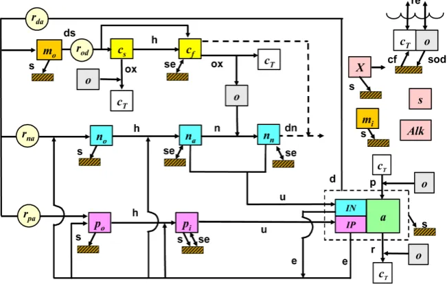
The algal model shows the sources and sinks of the water quality constituent, which are due to reactions and mass transfer mechanisms (Figure 3). The model documents sediment oxygen demand, whereby the sediment-water fluxes are

Figure 3. Schematic diagram of interacting water quality state variables in QUAL2Kw (ab

bottom algae, ap phytoplankton, mo detritus, cs slow CBOD, cf fast CBOD, cT total

inor-ganic carbon, O oxygen, nO organic nitrogen, na ammonia nitrogen, nn nitrite and nitrate

DOI:10.4236/jep.2019.1012097 1626 Journal of Environmental Protection documented according to the downward flux of particulate organic matter from the overlying water. Delivery of nitrogen, phosphorus and organic carbon to the anaerobic sediments are converted into inorganic phosphorus, dissolved me-thane and ammonium by mineralization, which are taken to the aerobic layer and oxidizing some of them, leading to sediment oxygen demand.

2.4.2. Processes

Several determinants are simulated as first-order decays, though nitrate, phosphate and DO are explained in more detail. The algal model for water quality variables interaction, is explained by Figure 3. The model comprises accumulation of detri-tus (mo), due to death of plants ( bottom algae and phytoplankton), dissolution and settling (Equation (24)). There is a gradual increase in reacting CBOD (CS) resulting from dissolution of detritus and is lost through oxidation and hydroly-sis (Equation (25)). Changes resulting from low oxygen Foxcf (denoted by F), is modeled by Equations (26a)-(26c) with the oxygen inhibition parameter Ksocf (denoted by K). Hydrolysis of slow reacting CBOD gives rise to the fast reacting CBOD (cf) and is lost through oxidation and denitrification (Equation (27)). Be-low are the equations representing Cs & Cf increase and loss, detritus (mo) ac-cumulation, and attenuation reactions

0 0

db b dt mo da dp p dt

k a v m

S r k a k m

H H

= + − − ₍₂₄₎

0 C 0

cs od di h s xcf dCs S

S =r k M −K C −F ⋅k c (25)

0 0

F k =

+ (half saturation) (26a)

(

)

1 exp

F= −_ − ⋅k o _ (exp) (26b) 2

2 0

0 F

k

=

+ (26c)

(

)

sti cf hc s oxcf dC f ondn oxndn dn n cH

i

A

S K C F k C r F k n J

v

= − − − + ₍₂₇₎

DOI: 10.4236/jep.2019.1012097 1627 Journal of Environmental Protection The concentration of organic nitrogen (no) rises as a result of plants death and is lost through hydrolysis and settling (Equation (28)). There is an increase in ammonia nitrogen(na) from hydrolysis of organic nitrogen and phytoplankton respiration and lost via photosynthesis and Nitrification (Equations (29a)-(29c)). There is a rise in nitrogen (nn) from the Nitrification of ammonia and us list via photosynthesis and denitrification (Equation (30)). Change in Nitrification re-sulting from reduced oxygen, Foxna (depicted as F) is represented by Equations (26a)-(26c) with ksona (depicted as K), which is an oxygen dependency parameter. The equations which involve nitrate nitrogen (nn), organic nitrogen (no), and ammonia nitrogen (na) are stated below.

(

)

0 0

n

bd b no na dp p N h

k a v n

S r k a q k n n

H H

 

= + _{ }− −

  (28)

(

)

(

)

4

0 0 0

botalguptakeN NupWcFrac

P

na hn xna na a na P p a ap P Np Lp p NH sti

ab

i

S k n F k n v F x K a r F kg a J

A p

v

γ η  φ φ 

= − + − _{ } +

− _ _ (29)

(

)(

)

(

)

(

)

ap

hnxp a hnxp n a n hnxp n

n k n n

P

k n k n n n k n

= +

+ + + + (29a)

(

)(

) (

)(

)

ab

hnxb a hnxb n a n hnxb n

n n n k

P

k n k n n n k n

= +

+ + + + (29b)

(

)

(

)

(

)

3

0 1 0

1 botalguptakeN NupWcFrac

nn xna na a xna dn n a ap P Np Lp p NO sti

ab

i

S F k n F k n r F kg a J

A p

v

η  φ φ 

= − − − _{ } +

 

−_ − _ (30)

where rna = ratio of nitrogen to chlorophyll a (mgN/mgA), khn = organic nitro-gen hydrolysis rate (1/day), kna = nitrification rate for ammonia nitrogen (1/day), krp = phytoplankton respiration rate (1/day), kgp = maximum photosyn-thesis rate at temperature (/d), kdp = phytoplankton death rate (/day), Foxna = at-tenuation due to low oxygen on ammonia nitrification (dimensionless), Foxp = attenuation due to low oxygen of phytoplankton respiration, von = organic ni-trogen settling velocity (m/d), qN = actual cell quotas of nitrogen (mgN/gD), NUpWCfrac = fraction of N uptake from the water column by bottom plants.

4

NH

J = sediment flux of ammonia (mgN/m2/day), BotAlgUptakeN = uptake

rate for nitrogen in bottom algae (mgN/m2_{/day) as defined in Equation (35f),}

3

NO

J is the sediment flux of nitrate (mgN/m2/day), A_st,i = the surface area of the

reach (m2_{), Pap = preferences for ammonium as nitrogen source for} phytoplank-ton, Pab = preferences for ammonium as nitrogen source for bottom algae, ΦNp = phytoplankton nutrient attenuation factor (dimensionless), ΦLp = phytoplankton light attenuation factor (dimensionless), khnxp = preferences coefficient of phy-toplankton for ammonium (mgN/m3_{), khnxb = preferences coefficient of bottom} algae for ammonium (mgN/m3_{) and k}

nn = temperature-dependent nitrification rate for ammonia nitrogen (1/day).

DOI:10.4236/jep.2019.1012097 1628 Journal of Environmental Protection the hydrolysis of organic phosphorus, and is lost via plant photosynthesis, set-tling and uptake of bottom algae (Equation (32)). There is an increase in organic phosphorus (po), resulting from plant death and is lost through hydrolysis and settling (Equation (31)). Inorganic suspended solids (mi) are lost through set-tling (Equation (33)). Loss and increase of phosphorus are represented by the equations,

(

)

0

0

0 0

a bd b

p Pa d p np

k a v p

S r k p P q k p p

H H

 

= +_{ } − −

  (31)

(

)

PO4

DOPHydr PhytoResp PhytoPhoto IPSettl

BotAlgUptakeP PUpWCfrac

pi pa pa

st i i

S r r

A J

V

= + − −

+_ − _ (32)

i mi i

v

S m

H

= (33)

where rpa = ratio of phosphorus to chlorophyll a (mgP/mgA), khp = organic phosphorus hydrolysis rate (/day), kdp = phytoplankton death rate (/day), qP = actual cell quotas of phosphorous (mgP/gD), vop = organic phosphorus settling velocity (m/day), vip = inorganic phosphorus settling velocity (m/day), vi = inor-ganic suspended solids settling velocity (m/day), PUpWCfrac = fraction of P uptake from the water column by bottom plants, JPO4 = the sediment flux of in-organic P (mgP/m2_{/day) and BotAlgUptakeP = uptake rate for phosphorous in} bottom algae (mgP/m2_{/day) as defined in Equation (35g).}

Phytoplankton (ap) increases due to photosynthesis and is lost via respiration, death and settling (Equations (34a)-(34e)). Michaelis-Menten equations (Equa-tion (34b)) are used to compute the nutrient attenua(Equa-tion factor φNp. Three mod-els (Equations (34c)-(34e)): half-saturation, Smith’s function and Steele’s equa-tions are combined with Beer-Lambert law to characterize the impact of light on phytoplankton photosynthesis (to estimate’ Lp) as,

0

P P

a

ap P N LP p xp p p dP p P

v

S kg a F k a k a a

H

γ

φ φ

= − − − _(34a)

*

2 3 3

*

2 3 3

H CO HCO

min , ,

H CO HCO

a n i Np

sNp a n sPp i sCp

n n p

k n n k p k

φ − −  ₊ _  _{ }+ _    =  + + + +_  _{ }+ _

  (34b)

( )

( )

0 1

ln

0 e e

Lp

Lp k H

e Lp

K I

k H K I

φ = _ + ₋ _

+

  (34c)

( )

( )

(

)

2 0 e 0 e e e k H Lp k H Lb I K I φ − − =

+ (smith 1932) (34d)

( )

1 0 e

e

k He e Lb I k H K Lb Lb I K φ − − ₊

= _{(steel 1962) (34e)}

DOI: 10.4236/jep.2019.1012097 1629 Journal of Environmental Protection half-saturation constant for phytoplankton (μg N/L), ksPp = phosphorus half-saturation constant for phytoplankton (μg N/L), ksCp = inorganic carbon half-saturation constant for phytoplankton (mole/L), KLp = light constant for phytoplankton (ly/day), and Ke = extinction coefficient, H CO2 *3 = sum of

dissolved CO2 and HCO3 (mg/m3/day).

Bottom algae (ab) increase due to photosynthesis and are lost via respiration and death (Equation (35a)). Attenuation due to low oxygen Foxb is modeled by Equations (26a)-(26c) with the oxygen inhibition parameter ksob. A logistic mod-el (Equation (35b)) is used to estimate space limitation attenuation factor φSb. The effect of nutrient limitation on bottom algae photosynthesis is modeled us-ing a formulation, accordus-ing to which the photosynthesis rate is dependent on intracellular nutrients (Equations (35c)-(35g)). The three models Equations (36a)-(36c), as in phytoplankton, are combined with Beer-Lambert law and in-tegrated to yield light attenuation factor φLb as given by equations,

(

)

(

)

,

PhytoPhoto-PhytoResp BotAlgPhoto-BotAlgResp

FastCOxid SlowCOxid NH4Nitr OxReaer

CODoxid SOD

st i

o oa od

i oc oc on

st i i

A

S r r

V

r r r

A V = + − − − + − − (35a)

where bottom algae photosynthesis (BotALgPhoto) can be modeled by two op-tions: 1) BotAlgPhoto 1/4 CgbfNbfLbfSbap (zero-order growth rate), where Cgb is the zero-order temperature/dependent maximum photosynthesis rate (gD/m2_{/day) and 2) BotAlgPhoto 1/4 CgbfNbfLbfSbab (first-order growth rate),} where Cgb = the first-order temperature-dependent maximum photosynthesis rate (day−1₎

,max 1 b Sb b a a

φ = − _(35b)

*

2 3 3

0

*

5 2 3 3

H CO HCO

min 1 1

9 H CO HCO

b

N

b

q p qN

N qp k c

φ − −    +       _     _ = _ − _ − _      + + 

  _{    } (35c)

b N b IN q a

= _(35d)

b P b IP q a

= _(35e)

(

)

BotAlgUptakeN a n qN

mN b

sNb a n qN N N

K

n n

a

k n n K q q

ρ +

=

+ + + − (35f)

(

)

BotAlgUptakeP i qP

mP b

sPb i qP P P

K p

a

k p K q q

ρ

=

+ + − (35g) The change in intracellular nitrogen and phosphorus in bottom algal cells are calculated respectively from Equations (35h) and (35i) as,

( )

BotAlgUptakeN BotAlgDeath

bN N N excb b

DOI:10.4236/jep.2019.1012097 1630 Journal of Environmental Protection

( )

BotAlgUptakeP BotAlgDeath

bP P P excb b

S = −q −q k T a (35i)

Following formulas are used for the bottom algae light attenuation coefficient:

( )

( )

0 e

0 e

e e

k H

Lb k H

Lb I

K I

φ = − ₋

+ (36a)

( )

( )

(

)

2 0 e

0 e

e

e

k H Lp

k H Lb

I

K I

φ −

−

=

+ (36b)

( )

1 0 e

e

k He e

Lb

I k H

K Lb

Lb

I

K

φ

−

− ₊

= _(36c)

where krb1 = temperature-dependent bottom algae basal respiration rate [/day], krb2 = bottom algae photo-respiration rate constant [dimensionless], Foxb = at-tenuation due to low oxygen on bottom algae respiration, krb Bottom algae res-piration rate (/day), ΦLb = bottom algae light attenuation factor (dimensionless), ΦNb = bottom algae nutrient attenuation factor (dimensionless), ΦSp = bottom algae space limitation factor (dimensionless), qN = cell quotas of nitrogen (mgN/gD), qP = cell quotas of phosphorus (mgP/gD), q0P = minimum cell quotas of phosphorus (mgP/gD), KLb = light constant for bottom algae (Ly/day), INb = intracellular nitrogen concentration (mgN/m2_{) and IPb = intracellular} phospho-rus concentration (mgP/m2_{). k}

sNb = nitrogen half-saturation constant for bottom algae (μg N/L), ksPb = phosphorus half-saturation constant for bottom algae (μg N/L), kscb = inorganic carbon halfsaturation constant for the bottom algae (mole/L), KqN = half-saturation constants for intracellular nitrogen (mgN/gD), KqP = half-saturation constants for intracellular phosphorus (mgP/gD), ρmN = maximum uptake rates for nitrogen in bottom algae (mgN/gD/day), ρmP = maximum uptake rates phosphorus in bottom algae (mgP/gD/day) and ab,max = carrying capacity (gA/m2_).

Pathogens (x) are lost due to death and settling (Equation (37)). Pathogens death is due to natural die-off and light and their death is modeled as a first-order temperature dependent decay. The death rate due to light is based on the Beer–Lambert law. The representing equation for pathogens is

( )

( )

(

)

1 e k He

dx path e

I

Sx k T x x

k H

α −

= + − ₍₃₇₎

DOI: 10.4236/jep.2019.1012097 1631 Journal of Environmental Protection

[

]

(

)

COD COD COD COD

v

S K

H

 

= − _{−  }

  (38)

where kCOD = COD oxidation rate (/day), vCOD = settling velocity of COD (m/day). Dissolved oxygen (O) increases due to photosynthesis and reaeration (Equations (39a)-(39c)). It is lost via CBOD oxidations, nitrification, plant res-piration, and oxidation of COD. The gain or loss of oxygen from atmosphere depends upon whether the water is under saturated or over saturated. The satu-ration concentsatu-ration depends upon local temperature and elevation above mean sea level (Equation (39c)). The reaeration rate ka is calculated using eight equa-tions available in the model which include: O’Connor-Dobbins, Churchill, Owens-Gibbs, Tsivoglou-Neal, Thackston-Dawson, USGS (pool-riffle), USGS (Channel control) and internal calculation. The effects of control structures are also included in the model. The equations involving dissolved oxygen (O) are:

(

)

(

)

,

PhytoPhoto-PhytoResp BotAlgPhoto-BotAlgResp

FastCOxid SlowCOxid NH4Nitr OxReaer

CODoxid SOD

st i

o oa o d

i oc oc on

st i i

A

S r r

V

r r r

A V

= +

− − − +

− −

(39a)

(

)

(

)

e 1 0.0001

Reaeration=k_a_ s − 148⋅elev −o _ (39b)

(

)

10 11

3 4

1.575701 10 6.642308 10

ln , 0 139.34411

1.243800 10 8.621949 10

s

a a

a a

o T

T T

T T

× ×

= − + −

× ×

+ −

(39c)

where ka = reaeration rate (1/day), Os = saturation concentration of dissolved oxygen (mgO2/L), Ta = absolute temperature (˚K), elev = elevation of the area (m), rod = ratio of oxygen consumed to detritus (mgO2/mgD) during bottom al-gae respiration, ron = ratio of oxygen consumed to nitrogen during nitrification (mgO2/mgN), roa = ratio of oxygen generated to phytoplankton growth (mgO2/mgA), roc = ratio of oxygen consumed during CBOD oxidation (mgO2/mgO2), Phytophoto = phytoplankton photosynthesis (gO2/m2/day), Phy-toResp = Phytoplankton respiration (gO2/m2/day), BotAlgPhoto = bottom algae photosynthesis (gO2/m2/day), BotAlResp = bottom algae respiration (gO2/m2/day), FastCOxid = fast CBOD oxidation (gO2/m2/day), SlowCOxid = slow CBOD oxidation (gO2/m2/day), NH4nitr = ammonium nitrification (gO2/m2/day), Reaeration = (gO2/m2/day) and CODoxid = oxidation of non-carbonaceous non-nitrogenous chemical oxygen demand (gO2/m2/day). The temperature effect for all first-order reactions used in the model is represented by:

( )

( )

20 T

k T =k θ − (40)

DOI:10.4236/jep.2019.1012097 1632 Journal of Environmental Protection 3 1 _* 2 3 HCO H H CO K − +         =  

  (41a)

2 3 2 3 CO H HCO K − + −         =  

  (41b)

H OH

w

K =    +  −_ (41c)

* 2

2 3 3 3

H CO HCO CO

T

c =_  _{ }+ − _{ }+ −_ (42)

10

pH= −log _H+_ (43)

where K1, K2, and Kw are acidity constants, Alk = alkalinity [eq L-1], H2CO3* = the sum of dissolved carbon dioxide and carbonic acid, HCO3

− _{= bicarbonate}

ion, 2 3

CO− = carbonate ion, H+ = hydronium ion, OH− = hydroxyl ion, and c_T =

total inorganic carbon concentration [mol/L]. The model accounts changes in alkalinity considering plant photosynthesis, respiration, nutrients hydrolysis, ni-trification, denini-trification, and bottom algae uptakes. It estimates total inorganic carbon, considering fast carbon oxidation, plant respiration, plant photosynthe-sis, and atmospheric aeration.

Temperature is modeled by performing a heat balance on each element i (Eq-uations (44a)-(44b)). The heat balance takes into account heat transfers from adjacent reaches, loads, abstractions, the atmosphere, and the sediments and in-cludes the influences of radiation, convection, and evaporation. The surface heat exchange Jh is modeled as a combination of five processes: solar shortwave radia-tion at the water surface I(0), atmospheric long wave radiaradia-tion Jan, long-wave back radiation from the water Jbr, conduction Jc, and evaporation Je (fluxes are expressed as cal/cm2_{/day) as represent by Equations (44a)-(44b)}

( )

h un br c e

J =I o +J −J −J −J (44a)

(

)

(

)

,

1 1

1 1 1

3

, , ,

6 3

d

d

m m m

100 cm 100 cm

10 cm

ab i

i i i i i

i i i i i i i

i i i i i

h i h i s i

w pw i w pw i w pw i

Q

T Q Q E E

T T T T T T T

t V V V V V

W J J

C V C H C H

ρ ρ ρ

− − − − + ′ ′ = − − + − + −       + _{ }+ _{ }+ _{ }       (44b)

where Ti = temperature in reach i (˚C), t = time (day), Ei′ = the bulk dispersion coefficient between reaches i and i + 1 (m3_{/day), Wh,I = the net heat load from point} and non-point sources into reach i (cal/day), ρw = the density of water (g/cm3), Cpw = the specific heat of water (cal/g˚C), Jh,i = the air-water heat flux (cal/cm2/day), Js,i = the sediment-water heat flux (cal/cm2_{/day), J}

s,i = sediment-water heat flux (cal/cm2_{/day) and ρ}

w = density of water (g/cm3). A complete discussion of the model theory is described by Pelletier and Chapra [26].

differ-DOI: 10.4236/jep.2019.1012097 1633 Journal of Environmental Protection ence between the model predictions and the observed data for water quality constituents. The genetic algorithm maximizes the fitness function f(x) as (Equ-ation (45)),

( )

(

)

1

0.5

1 1 ₂

2

m ij j m m

i i i

ij ij

m O

f x w

P O

=

= =

  

  

  

  

 

=_{   }

 

 _ − _ 

  

 

 _{ } _

 

∑

∑

∑

∑

where Oi,j = observed values, Pi,j = predicted values, m = number of pairs of pre-dicted and observed values, wi = weighting factors, and n = number of different state variables included in the reciprocal of the weighted normalized root mean squared error.

2.4.3. Input Data

Date, location, boundary conditions of flow, numerical integration control op-tions, headwater boundary flow and concentraop-tions, concentration for tributary point sources and diffuse sources, air temperature, hydraulic geometry (rating curve or Manning’s equation inputs for depth and velocity), shade, light attenu-ation parameters, reach segment lengths, options of solar radiattenu-ation, cloud cover, dew point temperature, long wave radiation, wind speed, evaporation, parame-ters to control the genetic algorithm for optional automatic calibration of water quality kinetics rates and constants, parameters for water quality kinetics rates and constants.

2.4.4. Model Capability

pH, temperature, conductivity, fast reacting CBOD, slow reacting CBOD, inor-ganic suspended solids, dissolved oxygen, orinor-ganic phosphorus, inorinor-ganic phos-phorus, ammonia nitrogen, organic nitrogen, nitrate nitrogen, pathogen, total organic carbon, bottom algae ( periphyton) nitrogen, bottom algae (periphyton) phosphorus, bottom algae (periphyton) biomass, detritus, phytoplankton, total inorganic carbon, alkalinity are all simulated by this model. It simulates only the main stream of a river and not its branches. Currently, it does not consistent an uncertainty component. It is a steady-flow, 1D model and is unable to assess va-riable flow.

2.4.5. Strengths and Its Application

The QUAL2KW is able to derive carbonaceous Biochemical Oxygen demand, via the conversion of algal death [19][20]. Therefore, where macrophyte (rooted aquatic plants) serve a unique purpose, this model is suitable. It is well detailed and available. It is made up of automatic calibration system. This model has been used on the south Umpqua river, Oregon, USA to assess the dissolved oxygen

DOI:10.4236/jep.2019.1012097 1634 Journal of Environmental Protection temperature, pH and nutrients in the Wenatchee River, Washington state [31].

2.5. WASP7

WASP7 [32] is a modernized version of the original WASP [33][34][35][36], which is found free in the United States Environmental Protection Agency’s website http://www.epa.gov/athens/wwqtsc/. The development of this model began in the 1970’s [37]. The WASP can be seen as a dynamic compart-ment-modeling program for aquatic systems, the water column and underlying benthos both inclusive. The following processes change with time, and they in-clude: dispersion, point and diffuse mass loading, advection-dispersion and boundary exchange are simulated in the basic program. 1, 2, and 3 dimensional systems and different types of pollutant can be assessed using WASP7. It is use-ful in assessing different problems of water quality in various water bodies such as, streams, rivers, coastal waters, ponds, estuaries, lakes, and reservoirs. It is as-sociated with sediment transport models and hydrodynamic models (like EFDC, DYNHYD; environmental fluid Dynamics code), which provides salinity, flows, sediment fluxes, temperature and depth velocities. It contains

• _{High speed WASP7 sub-model processors.} • _{Easily accessible Windows-based interface.}

• _{A pre-processor to aid in processing of data into a format which can be used}

in WASP7.

• _{Graphical postprocessor to enable viewing of the WASP7 results.}

The old versions of WASP have two general kinetic modules [33]: EUTRO for conventional water quality and TOXU for toxicants. Advanced sub-models of EUTRO (named periphyton), HEAT and MECURY were added for particular modeling needs. This provided a medium for Simulation of periphyton (at-tached bottom algae) with nutrients uptake. Routines in the QUAL2K model contain algorithms which assess changes in concentration of periphyton and de-tritus [27]. The kinetic sub-models TOXI and EUTRO can aid in simulation of two major types of water quality problems: toxic pollution (with sediments, or-ganic chemicals and metals) and conventional pollution (with Biochemical oxy-gen demand, dissolved oxyoxy-gen, eutrophication and nutrients). The EUTRO can be utilized at different complex levels to simulate the variables and interactions. About three types of particulate material and about three chemicals have been simulated by TOXI. The chemicals may be associated with reaction yields or may not. Any of the chemicals being simulated, may present in five ways:

1) Doubly charged cations. 2) Singly charged cations. 3) Doubly charged anions. 4) Singly charged anions. 5) Neutral molecules.

DOI: 10.4236/jep.2019.1012097 1635 Journal of Environmental Protection 2) Sorbed to dissolved organic carbon (DOC).

3) Sorbed to the three different solids types.

Therefore, 25 forms of each chemical can be modeled in TOXI. Ambrose et Al

[32] and Wool et al. [33] contain a well detailed documentation.

2.5.1. Conceptualization

This model is based on compartmentalization principle. For each equation, a mass balance equation is stated out. Within each compartment, there us rapid and complete mixing. WASP7 solves the equations according to the conserva-tion of mass principle. The three main classes of water quality processes (load-ing, transformation and transportation), are represented by these equations. Out of these three processes, about three components play a major role with concen-tration variability along the river reach, and these processes include: dispersion, advection-dispersion and kinetic transformation (biological, physical and chem-ical transformation). WASP7 assessed every component of water quality from the point of temporal and spatial input to the point of export and conserving mass in space and time, which is its final point. A finite-difference equation is used for every segment, when temporal and spatial variations in concentration of the constituent are being accounted for. For easy use, derivation of the finite difference form of the equation of mass balance is for a 1D reach. For every segment, the concentration is calculated. The final concentration which is de-rived from the previous segment is the initial value used for each segment at time zero. In a body of water, the dissolved components representing the three main grades of water quality processes-transport (term 1), loading (term 2) and transformation (term 3), the equation of mass balance is (Equation (46)):

( )

( )

₍

₎

x x L B k

AC C

u AC E A A S S AS

t x t

∂ ∂  ∂ 

= − + + + +

∂ ∂ _ ∂ _ (46)

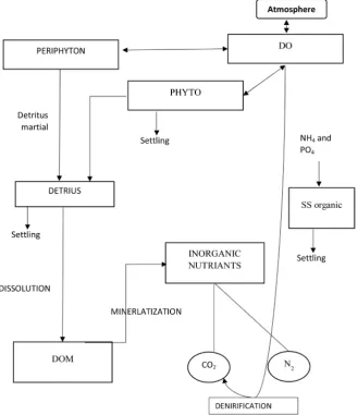
where C is concentration of water quality (g/m3_{), t is time (day), Ux is} longitu-dinal velocity (m/day), Ex is longitudinal diffusion coefficient (m2/day), SL is dif-fusion loading rate (g/m3 _{day), SB is boundary loading rate including upstream,} downstream, benthic, atmospheric (g/m3 _{day), Sk = transformation term (total} kinetic transformation rate; positive is source, negative is sink, g/m3 _{day for} va-riable i in a segment) and A is cross-sectional area (m2_{). The physical and} chem-ical processes, that affect the transport and interaction among the nutrients, phytoplankton, carbonaceous material, sediment, atmosphere and dissolved oxygen in the aquatic environment, is shown in Figure 4.

2.5.2. Processes

DOI:10.4236/jep.2019.1012097 1636 Journal of Environmental Protection Dissolved oxygen (DO): anaerobic processes in the underlying sediments and aerobic respiratory processes in the water column results in a decrease in DO. Phytoplankton growth, re-aeration result in increase in DO and sediment oxy-gen demand, phytoplankton respiration and oxidation of CBOD result in loss of DO (Equation (47)):

Figure 4. State variable interactions in advanced eutrophication submodel in WASP7 (Phyto is phytoplankton as carbon, NO3 is nitrate, NH4 is ammonium, PO4 is

or-tho-phosphorus, CBOD is carbonaceous biochemical oxygen demand, DO is dissolved oxygen ON is organic nitrogen, OP is organic phosphorous, DOM is dissolved organic matter, SS is inorganic suspended solids) [36].

(

)

(

)

1 3 1

6

6 1

6

4 4

32 48 14 32

1

12 14 12 12 R

b

a sat d

BOD

P NH

c C SOD

k c c k c

t k C D

G P c k c

 

∂

= − − _{ } −

∂ _ + _

 

+ _ + − _ −

 

(47)