Volume 8, 2018, Pages 11–23 TNC’18. Trusted Numerical Computations
Improving the Numerical Accuracy of High Performance
Computing Programs by Process Specialization
Farah Benmouhoub, Nasrine Damouche, and Matthieu Martel
LAMPS Laboratory University of Perpignan,
52 Avenue Paul Alduy, Perpignan, France, 66860.
{first.last}@univ-perp.fr
Abstract
In high performance computing, nearly all the implementations and published experi-ments use floating-point arithmetic. However, since floating-point numbers are finite ap-proximations of real numbers, it may result in hazards because of the accumulated errors. These round-off errors may cause damages whose gravity varies depending on the critical level of the application. To deal with this issue, we have developed a tool which im-proves the numerical accuracy of computations by automatically transforming programs in a source-to-source manner. Our transformation, relies on static analysis by abstract interpretation and operates on pieces of code with assignments, conditionals, loops, func-tions and arrays. In this article, we apply our techniques to optimize a parallel program representative of the high performance computing domain. Parallelism introduces new nu-merical accuracy problems due to the order of operations in this kind of systems. We are also interested in studying the compromise between execution time and numerical accuracy.
1
Introduction
The IEEE754 Standard [1,23] specifies the floating-point number arithmetic which is more and more used in many industrial domains including numerical simulations. However, floating-point arithmetic is prone to accuracy problems due to the round-off errors. The round-off errors which may be introduced by the approximation, can generate catastrophic results like the destruction of the British Petroleum plateform [27].
transformation. This is possible thanks to the set of intraprocedural and interprocedural trans-formation rules defined in previous work [10, 9]. Salsa relies on static analysis by abstract interpretation [4] to compute variable ranges and round-off error bounds.
In this article, we are interesting in applying our techniques in order to improve the numerical accuracy of high performance computing programs. More precisely, we aim at taking advantage of the fact that each process may execute the operation in its own order. In other words, the idea is to pass from a hand-written SPMP code to a synthesized MIMD code in which each process is specialized with respect to its data. To do this, we have taken an example of application that simulates the propagation of heat in a grid, implemented with theMPIlibrary.
We present a comprehensive summary of howSalsaworks. An extended description is given in [10]. We give an overview of the formal intraprocedural [9] and interprocedural [10] rules used in our transformation as well as on how the transformation of expressions is done [20].
The article is organized as following. Section 2 describes related work. In Section 3, we present the IEEE754 Standard and how to compute the error bounds, we give also a brief description of how transforming arithmetic expressions, intraprocedural and interprocedural programs. Section 4 details our motivation example and describe how we have proceeded in our experimentations. Section5 describes the experimental results obtained when measuring the numerical accuracy of programs. In Section 6, we give numbers on the execution time required by programs before and after being optimized. Section7 concludes.
2
Related Work
Several static analyses of the numerical accuracy of floating-point computations have been introduced during these last years. These methods over-approximate the worst error arising during the executions of a program. Static analyses based on abstract interpretation [4,5] have been proposed and implemented in theFluctuattool [17,18] which has been used in several industrial contexts. A main advantage of this method is that it enables one to bound safely all the errors arising during a computation, for large ranges of inputs. It also provides hints on the sources of errors, that is on the operations which introduce the most important precision loss. This latter information is of great interest to improve the accuracy of the implementation. More recently, Darulova and Kuncak have proposed a tool,Rosa, which uses a static analysis coupled to a SMT solver to compute the propagation of errors [12]. Solovyev et al. have proposed another tool, FP-Taylor based on symbolic Taylor expansions [26]. None of the techniques mentioned above generate more accurate programs.
Other approaches rely on dynamic analysis. For instance, the Precimonious tool tries to decrease the precision of variables and checks whether the accuracy requirements are still full filled [2]. Lam et al. instrument binary codes in order to modify their precision without modifying the source codes [21]. They also propose a dynamic search method to identify the pieces of code where the precision should be modified. Again, these techniques do not transform the codes in order to improve the accuracy.
3
Background
In this section, we first present the floating-point arithmetic and then how round-off errors are computed. Second, we briefly describe how to transform arithmetic expressions in order to improve their numerical accuracy [20]. Finally, we give the principles of the transformation of both intraprocedural and interprocedural programs implemented in our tool,Salsa.
3.1
Floating-Point Arithmetic
In this section, we start by giving a brief description of the IEEE754 Standard [1] and then we present how to compute the round-off errors.
3.1.1 The IEEE754 Standard
Floating-point numbers are used to represent real numbers [1, 15]. Because of their finite representation, round-off errors arise during the computations and this may cause damages in critical contexts. The IEEE754 Standard formalizes a binary floating-point number as a triplet made of a sign, a mantissa and an exponent. We consider that a numberxis written:
x=s·(d0.d1. . . dp−1)·be=s·m·be , (1)
where,sis the sign∈ {−1,1},bis the basis (b= 2),mis the mantissa,m=d0.d1. . . dp−1with
digits 0≤di < b, 0≤i≤p−1,pis the precision andeis the exponent e∈[emin, emax]. The IEEE754 Standard specifies some particular values forp,emin andemax.
The IEEE754 Standard defines four rounding modes for elementary operations over floating-point numbers. These modes are towards−∞, towards +∞, towards zero and to the nearest respectively denoted by↑+∞,↑−∞,↑0 and↑∼. LetRbe the set of real numbers andFbe the
set of floating-point numbers (we assume that only one format is used at the time, e.g. single or double precision). The semantics of the elementary operations specified by the IEEE754 Standard is given by Equation (2).
x~ry=↑r(x∗y) , with ↑r:R→F , (2)
where a floating-point operation, denoted by ~r, is computed using the rounding mode r ∈
{↑+∞, ↑−∞, ↑0, ↑∼} and ∗ ∈ {+,−,×,÷} is an exact operation. Obviously, the results of the computations are not exact because of the round-off errors. This is why, we use also the function↓r:R→Rthat returns the round-off error. We have
↓r(x) =x− ↑r(x) . (3)
3.1.2 Error Bound Computation
In order to compute the errors during the evaluation of arithmetic expressions [22], we use values which are pairs (x, µ) ∈ F×R ≡E where x is the floating-point number used by the
machine and µ is the exact error attached to F, i.e., the exact difference between the real and floating-point numbers as defined in Equation (3). For example, the real number 1
3 is
represented by the valuev= (↑∼ 13,↓∼ 31) = (0.333333,(13−0.333333)). The semantics of the elementary operations onEis defined in [22].
Our tool uses an abstract semantics [4] based onE. The abstract values are represented by a
pair of intervals. The first interval contains the range of the floating-point values of the program and the second one contains the range of the errors obtained by subtracting the floating-point values from the exact ones. In the abstract value (x],µ])∈
to the range of the values andµ] is the interval of errors on x]. This value abstracts a set of concrete values{(x, µ) : x∈x] and µ∈µ]} by intervals in a component-wise way. We now introduce the semantics of arithmetic expressions onE]. We approximate an intervalx] with real bounds by an interval based on floating-point bounds, denoted by ↑] (x]). Here bounds are rounded to the nearest, see Equation (4).
↑]([x, x]) = [↑∼(x),↑∼(x)] . (4)
We denote by↓] the function that abstracts the concrete function↓
∼. Every error associated tox∈[x, x] is included in↓]([x, x]). For a rounding mode to the nearest, we have
↓]
([x, x]) = [−y, y] with y=1
2ulp max(|x|,|x|)
. (5)
Formally, the unit in the last place, denoted by ulp(x), consists of the weight of the least significant digit of the floating-point numberx. Equations (6) and (7) give the semantics of the addition and multiplication overE], for other operations see [22]. If we sum two numbers, we
must add the errors on the operands to the error produced by the round-off of the result. When multiplying two numbers, the semantics is given by the development of (x]1+µ]1)×(x]2+µ]2).
(x]1, µ]1) + (x]2, µ]2) = ↑]
(x]1+x]2), µ]1+µ]2+↓]
(x]1+x]2)
, (6)
(x]1, µ]1)×(x]2, µ]2) = ↑]
(x]1×x]2), x]2×µ]1+x]1×µ]2+µ]1×µ]2+↓]
(x]1×x]2)
. (7)
3.1.3 Transformation of Expressions
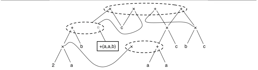
We briefly introduce former work [20,28] to semantically transform arithmetic expressions using Abstract Program Expression Graph (APEG). This data structure remains in polynomial size while dealing with an exponential number of equivalent arithmetic expressions. To prevent any combinatorial problem, APEGs hold in abstraction boxes many equivalent expressions up to associativity and commutativity. A box containing n operands can represent up to 1×3×5...×(2n−3) possible formulas. In order to build large APEGs, two algorithms are used (propagation and expansion algorithms). The first one searches recursively in the APEG where a symmetric binary operator is repeated and introduces abstraction boxes. Then, the second algorithm finds a homogeneous part and inserts a polynomial number of boxes. In order to add new shapes of expressions in an APEG, one propagates recursively subtractions and divisions into the concerned operands, propagate products, and factorizes common factors. Finally, an accurate formula is searched among all the equivalent formulas of the APEG using the abstract semantics of Section3.1.2.
Example 3.1. An example of APEG is given in Figure1. When an equivalence class (denoted by a dotted ellipse) contains many sub-APEGsp1, . . . , pn then one of the pi, 1≤i≤n, must
be selected in order to build an expression. A box ∗(p1, . . . , pn) represents any parsing of the expression p1∗. . .∗pn. For instance, the APEG p of Figure 1 represents all the following
expressions:
A(p) =
( (a+a) +b
×c, (a+b) +a
×c, (b+a) +a
×c, (2×a) +b
×c,
c× (a+a) +b
, c× (a+b) +a
, c× (b+a) +a
, c× (2×a) +b
, (a+a)×c+b×c, (2×a)×c+b×c, b×c+ (a+a)×c, b×c+ (2×a)×c
)
.
3.1.4 Intraprocedural and Interprocedural Transformation
In this section, we introduce our tool Salsa for numerical accuracy optimization by program transformation. Salsa is a tool that improves the numerical accuracy of programs based on floating-point arithmetic [6]. It reduces partly the round-off errors by automatically trans-forming C programs in a source-to-source manner. We have defined a set of intraprocedural transformation rules [9] like assignments, conditionals, loops, etc., and interprocedural trans-formation rules [10] for functions and other rules which deal with arrays. These rules have been implemented in theSalsatool. Salsarelies on static analysis by abstract interpretation to compute variable ranges and round-off error bounds. it takes as first input ranges for the input variables of programs id ∈ [a, b]. These ranges are given by the user or coming from sensors. Salsatakes as second input a program to be transformed. Salsaapplies the required transformation rules and returns as output a transformed program with better accuracy.
Salsais composed of several modules. The first module is the parser that takes the original program in C language with annotations, puts it in SSA form (Static Single Assignment form) and then returns its binary syntax tree. The second module consists in a static analyzer, based on abstract interpretation [4], that infers safe ranges for the variables and computes errors bounds on them. The third module contains the intraprocedural transformation rules. The fourth module implements the interprocedural transformation rules. The last module is the Sardana tool, that we have integrated in our Salsa and call it on arithmetic expressions in order to improve their numerical accuracy.
When transforming programs we build larger arithmetic expressions that we choose to parse in a different ways to find a more accurate one. These large expressions will be sliced at a given level of the binary syntactic tree and assigned to intermediary variables namedTMP. Note that the transformed program is semantically different from the original one but mathematically are equivalent. In [8], we have introduced a proof by induction that demonstrate the correctness of our transformation. In other words, we have proved that the original and the transformed programs are equivalent.
In practice, our transformation performs states of the formhc, δ, C, ν, βiwhere:
• c is a command,
• δ is a formal environment which maps variables to expressions. Intuitively, this envi-ronment records the expressions assigned to variables in order to inline them later on in larger expressions,
• C is a single hole context [19] that records the program enclosing the current command
2 a
×
+
b
□
+(a,a,b)
×
c ×
+
c b c
×
a a
+
×
× +
to be transformed,
• ν denotes thetarget variable that we aim at optimizing,
• β consists in a black list that contains the list of the variables that we must not remove from the program. Initially,β containsν,i.e., thetarget variable νmust not be removed.
Example 3.2. For example, let us consider the program in Figure 2 with a conditional. We assume thatν=zis the variable that we aim at optimizing. Initially, in the top left of Figure2, the environmentδand the contextCare empty and the black listβcontains the target variablez. The first line of the program is an assignment, so we have rules that remove the assignments from the program and saving them into the memory δ when some conditions are verified. So, the first step, consists in removing the variableaand memorizing it inδ. Consequently, the line corresponding to the variable discarded is replaced bynop, the new environment is δ= [x7→a]
and the context contains the assignment discard, i.e., C = x = a. The new intermediary program is given in the top right of Figure2. Next, we apply rules for sequences of commands and then we discard the noplines from the program. The next step consists in analyzing this new program. We remark that the variable x is undefined in our program, this is why, we reinsert it into the program as given in the bottom left of Figure2. Consequently, we remove it from the memoryδand we add it to the black listβ. Now, to transform the conditional block of program, we dispose of several rules that transform only the executed branch if the evaluation of the condition is statically known, otherwise, we transform both branches of the conditional. In our case, we transform thethen and theelse branches using partial evaluation rules. The final program is shown in the bottom right of Figure2.
4
Case Study
In this section, we describe our case study to demonstrate thatSalsa improves the numerical accuracy of the floating-point computations performed by a parallel code written in MPI [25]. The considered application models the temperature spread of a rectangular plate initially heated at two corners. For the simulations, we consider a grid of size [X×Y], which temperature is initialized to the value of 0.1 and heated at the top left and bottom right corners. In our experiments, we aim at performing a fast and accurate computation of the propagation of the heat on the grid. We use a parallel code in which we split the grid into bands, so that these bands can be assigned to different computational nodes, which can then work in parallel. Then, the parallelization is done by sharing the array representing the grid between working nodes as shown in the Figure 3. For this, we have to count our working nodes and distribute the data among them. Since, the nodes need neighbor line data to calculate their own line data, the values on the borders have to be communicated between the nodes. This is done with MPI Send() and MPI Rec(), that are included in the MPI environment.
Independently of the analytical solution, we can give a numerical solution to this problem as well. This solution consists in an iterative computation, where current heat values are used for calculating the new heat values in the grid. The propagation of the heat at every point of the grid is calculated by the average of the heat of points that surround it. This average will be the new heat value of the current point, for example the case of a point in the center of the grid with stencil equal to one, see Equation (8).
new[i][j] =old[i−1][j] +old[i+ 1][j] +old[i][j−1] +old[i][j+ 1]
4 . (8)
δ=∅
C= [] β={z}
x = a ;
if ( x > 3.) t h e n z = x + 2. + 1. ; e l s e
z = x - 2. - 1. ;
δ0=δ[x7→a] C=x=a; [] β={z}
nop ;
if ( x > 3.) t h e n z = x + 2. + 1. ; e l s e
z = x - 2. - 1. ;
δ0=∅
C= [] β={x, z}
x = a ;
if ( x > 3.) t h e n z = x + 2. + 1. ; e l s e
z = x - 2. - 1. ;
δ0=∅
C=x=a; if(x >3) then [] else [] β={x, z}
x = a ;
if ( x > 3.) t h e n z = x + 3. ; e l s e
z = x - 3. ;
Figure 2: Initial (top left) program. First intermediary transformed (top right) program. Second intermediary transformed (bottom left) program. Final transformed (bottom right) program.
PROCESSOR 2
PROCESSOR 3 PROCESSOR 0
PROCESSOR 1 200
400
800 600
0 T°
T°
Figure 3: View of grid [800×800] partitioning according to the number of processors in this case 4 processors (left), example of the points involved when calculating heat at a point(right).
• The first one consists in increasing the stencil and observing the impact of the stencil on the spread of the heat in our grid. Equation (9) defines the computations of the heat at the center when the stencil is equal to two.
• The second parameter concerns the variation of the initial heat value at the two corners (top left and bottom right) according to significant melting temperatures of the chemical elements like Iron which is equal to 2800.4◦F, Platinum equal to 3214.76◦F, Copper equal to 1984.316◦F and Calcium 1547.6◦F.
• The last parameter is to change the number of iterations in order to find out if we run the simulation long enough, so that the temperature of the heated corners reaches all points of the grid.
5
Numerical Accuracy
In this section, we present the experimental results of our study concerning the numerical accuracy of computations. First, we study the impact of the propagation of the heat when increasing the stencil on the grid. To be done, we have to consider a parallel program with MPI [25]. The result of this simulation is given in Figure4.
Figure 4: View of the heated grid at the two corners, number of iterations: 3600, stencil: 1 (left), stencil: 2 (right).
We notice that the figure has a blur effect at the corners which is due to the applied heating value. Thus, the initial temperature propagates inside the grid. If we run the program long enough (increasing the number of iterations), the value of the heated corners reaches all points of the grid.
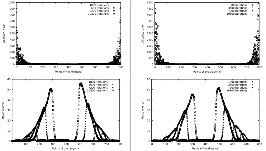
Figure 5: Absolute error between original program and optimized program, initial temperature: 10106.6◦F, number of iterations: 1800 (top left), 3600 (top right), 7200 (bottom left), 10800 (bottom right).
the program of each processor according to its data. In the case of processor 0, Equation (8) becomes Equation (10):
new[i][j] =(((old[i][j+ 1] +old[i+ 1][j]) +old[i−1][j]) +old[i][j−1])
4 . (10)
of the form of Equation (11):
new[i][j] =(old[i][j+ 1] + (old[i+ 1][j] + (old[i][j−1] +old[i−1][j])))
4 . (11)
Figures 5and6 respectively, represent the relative and absolute error on the computations of the heat propagation on a grid of dimension [800×800], heated on the top left and bottom right corners at a temperature equal to that of platinum fusion.
On the one hand, if we are interested in the absolute errors on Figure5, we notice that they are negligible in the middle of the grid, since we have not iterated enough on the computations of the heat propagation, so that the errors reach these points of the grid. We also notice that the absolute errors around the corners corresponding to the heating points appear small at the beginning for a number of iterations equal to 1800 top left on Figure5. These errors will be accumulated and propagated while increasing the number of iterations such that it is presented in Figure 5 (3600 iterations top right, 7200 iterations bottom left, 10800 iterations bottom right). In addition, when we measure the execution time corresponding to each case of the iterations number previously presented in Figure5, we note that it takes only 0.52 seconds to do 1800 iterations and it needs 1.14 seconds to obtain 10800 iterations.
On the other hand, if we are interested in the relative errors of Figure 6, we notice the presence of errors around the heating corners. These errors depend on the number of iterations as well as the initial heating value of the two corners.
0 100 200 300 400 500 600 700 800 900 1000
0 100 200 300 400 500 600 700 800
A b so lu te e rr o r
Points of the diagonal
1800 iterations 3600 iterations 7200 iterations 10800 iterations 0 500 1000 1500 2000 2500 3000 3500 4000 4500 5000
0 100 200 300 400 500 600 700 800
A b so lu te e rr o r
Points of the diagonal
1800 iterations 3600 iterations 7200 iterations 10800 iterations 0 10 20 30 40 50 60
0 100 200 300 400 500 600 700 800
R e la ti ve e rr o r
Points of the diagonal
1800 iterations 3600 iterations 7200 iterations 10800 iterations 0 10 20 30 40 50 60
0 100 200 300 400 500 600 700 800
R e la ti ve e rr o r
Points of the diagonal
1800 iterations 3600 iterations 7200 iterations 10800 iterations
Initial Nbre of Iterations Nbre of Iterations Exec. Time Exec. Time temperature before transfo. after transfo. before transfo. after transfo.
1010.6◦ 10945 10912 1.110s 1.080s
1547.6◦ 6712 6693 0.916s 0.901s
1984.316◦ 5426 5411 0.876s 0.867s
2800.4◦ 3652 3643 0.797s 0.814s
3214.6◦ 3202 3190 0.789s 0.778s
10106.6◦ 1303 1290 0.716s 0.705s
Figure 7: Measurement of number of iterations and execution time of program of Section4.
6
Execution Time
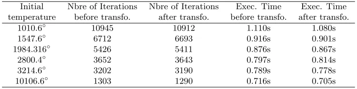
In this section, we extend the concept proved bySalsaon accelerating the convergence speed [7] of serial programs to parallel programs. In practice, we have applied this study on the program of heat propagation previously described in Section4. The results obtained when transforming the program with Salsa show that the numerical accuracy and the execution time of the program have been improved and the convergence speed has been accelerated, more precisely, the number of iterations required to converge to a given value has been reduced (this value consists in the middle point of the grid). Figure7 summarizes the different results in terms of number of iterations and execution time obtained when varying the initial temperature of the grid before and after the transformation.
If we take the example of a temperature that equal to 1010.6◦, we want to calculate the number of iterations necessary to reach the value of 357◦in the middle of the grid. Our results show that we are reducing the number of iterations of 33 iterations.
7
Conclusion
References
[1] ANSI/IEEE. IEEE Standard for Binary Floating-Point Arithmetic. SIAM, 2008.
[2] F. Benz, A. Hildebrandt, and S. Hack. A dynamic program analysis to find floating-point accuracy problems. InProgramming Language Design and Implementation, PLDI ’12, 2012, pages 453–462. ACM, 2012.
[3] J. Bertrane, P. Cousot, R. Cousot, F. Feret, L. Mauborgne, A. Min´e, and X. Rival. Static analysis by abstract interpretation of embedded critical software. ACM SIGSOFT Software Engineering Notes, 36(1):1–8, 2011.
[4] P. Cousot and R. Cousot. Abstract interpretation: A unified lattice model for static analysis of programs by construction or approximation of fixpoints. InPrinciples of Programming Languages, pages 238–252, 1977.
[5] P. Cousot and R. Cousot. Systematic design of program transformation frameworks by abstract interpretation. InPrinciples of Programming Languages, pages 178–190. ACM, 2002.
[6] N. Damouche and M. Martel. Salsa : An automatic tool improve the accuracy of programs. In 6th International Workshop on Automated Formal Methods, AFM, 2017.
[7] N. Damouche, M. Martel, and A. Chapoutot. Impact of accuracy optimization on the convergence of numerical iterative methods. In M. Falaschi, editor, LOPSTR 2015, volume 9527 of Lecture Notes in Computer Science, pages 143–160. Springer, 2015.
[8] N. Damouche, M. Martel, and A. Chapoutot. Data-types optimization for floating-point formats by program transformation. InInternational Conference on Control, Decision and Information Technologies, CoDIT 2016, Saint Julian’s, Malta, April 6-8, 2016, pages 576–581, 2016.
[9] N. Damouche, M. Martel, and A. Chapoutot. Improving the numerical accuracy of programs by automatic transformation. In International Journal on Software Tools for Technology Transfer, volume 19, pages 427–448. Springer, 2016.
[10] N. Damouche, M. Martel, and A. Chapoutot. Numerical accuracy improvement by interprocedural program transformation. In Sander Stuijk, editor,Proceedings of the 20th International Workshop on Software and Compilers for Embedded Systems, SCOPES 2017, Sankt Goar, Germany, June 12-13, 2017, pages 1–10. ACM, 2017.
[11] N. Damouche, M. Martel, P. Panchekha, C. Qiu, A. Sanchez-Stern, and Z. Tatlock. Toward a standard benchmark format and suite for floating-point analysis. In P. Prabhakar S. Bogomolov, M. Martel, editor,NSV’16, Lecture Notes in Computer Science. Springer, 2016.
[12] E. Darulova and V. Kuncak. Sound compilation of reals. In S. Jagannathan and P. Sewell, editors, POPL’14, pages 235–248. ACM, 2014.
[13] D. Delmas, E. Goubault, S. Putot, J. Souyris, K. Tekkal, and V. V´edrine. Towards an industrial use of FLUCTUAT on safety-critical avionics software. InFormal Methods for Industrial Critical Systems, volume 5825 ofLecture Notes in Computer Science, pages 53–69. Springer, 2009. [14] P-L. Garoche, F. Howar, T. Kahsai, and X. Thirioux. Testing-based compiler validation for
synchronous languages. In J. M. Badger and K. Yvonne Rozier, editors,NASA Formal Methods -6th International Symposium, NFM 2014, Proceedings, volume 8430 ofLecture Notes in Computer Science, pages 246–251. Springer, 2014.
[15] D. Goldberg. What every computer scientist should know about floating-point arithmetic. ACM Comput. Surv., 23(1):5–48, 1991.
[16] E. Goubault. Static analysis by abstract interpretation of numerical programs and systems, and FLUCTUAT. In Static Analysis Symposium, SAS, volume 7935 of Lecture Notes in Computer Science, pages 1–3. Springer, 2013.
Computer Science, pages 209–212. Springer, 2002.
[18] E. Goubault, M. Martel, and S. Putot. Some future challenges in the validation of control systems. InEuropean Congress on Embedded Real Time Software, ERTS 2006, Proceedings, 2006.
[19] E. Hankin. Lambda Calculi A Guide For Computer Scientists. Clarendon Press, Oxford, 1994. [20] A. Ioualalen and M. Martel. A new abstract domain for the representation of mathematically
equivalent expressions. InSAS’12, volume 7460 ofLNCS, pages 75–93. Springer, 2012.
[21] M. O. Lam, J. K. Hollingsworth, R. Bronis, and M. P. LeGendre. Automatically adapting programs for mixed-precision floating-point computation. InSupercomputing, ICS’13, pages 369–378. ACM, 2013.
[22] M. Martel. Semantics of roundoff error propagation in finite precision calculations. Higher-Order and Symbolic Computation, 19(1):7–30, 2006.
[23] J. M. Muller, N. Brisebarre, F. De Dinechin, C-P. Jeannerod, V. Lef`evre, G. Melquiond, N. Revol, D. Stehl´e, and S. Torres. Handbook of Floating-Point Arithmetic. Birkh¨auser, 2010.
[24] J. R. Wilcox P. Panchekha, A. Sanchez-Stern and Z. Tatlock. Automatically improving accuracy for floating point expressions. InPLDI’15, pages 1–11. ACM, 2015.
[25] P. Pacheco. An Introduction to Parallel Programming. Morgan Kaufmann Publishers Inc., San Francisco, CA, USA, 1st edition, 2011.
[26] A. Solovyev, C. Jacobsen, Z. Rakamaric, and G. Gopalakrishnan. Rigorous estimation of floating-point round-off errors with symbolic taylor expansions. InFM’15, volume 9109 ofLNCS, pages 532–550. Springer, 2015.
[27] G. Suzanne and M. Terry. Bp suspended from new us federal contracts over deepwater disaster, 2012.
![Figure 3: View of grid [800×800] partitioning according to the number of processors in thiscase 4 processors (left), example of the points involved when calculating heat at a point(right).](https://thumb-us.123doks.com/thumbv2/123dok_us/8878199.1818113/7.612.102.513.101.344/figure-partitioning-according-processors-thiscase-processors-involved-calculating.webp)