COMBINING GENETIC ALGORITHM AND SINC-GALERKIN METHOD FOR SOLVING AN INVERSE DIFFUSION PROBLEM

(1)

HASSAN DANA MAZRAEH1, REZA POURGHOLI1, TAHEREH HOULARI1, §

Abstract. A numerical approach combining the use of a genetic algorithm with the solution of the Sinc-Galerkin method is proposed for the determination of an unknown time-dependent diffusivitya(t) in an inverse diffusion problem (IDP). At the beginning of the numerical algorithm, Sinc-Galerkin method is employed to solve the direct diffusion problem. The present approach is to rearrange the matrix forms of the governing equa-tions. Then, the genetic algorithm is adopted to find the solution of IDP. The genetic algorithm used in this work is not a classical genetic algorithm. Instead, the applica-tion of the genetic algorithm to this discrete-time optimal control problem is called a real-valued genetic algorithm(RVGA). Some numerical experiments confirm the utility of this algorithm as the results are in good agreement with the exact data. Results show that a reasonable estimation can be obtained by combining the genetic algorithm and Sinc-Galerkin method within a CPU with clock speed 2.7 GHz.

Keywords: Inverse diffusion problem, genetic algorithm, Sinc-Galerkin method. AMS Subject Classification: 65M32, 35K05.

1. Introduction

Solution of an inverse diffusion problem requires to determine an unknown diffusion co-efficient from an additional information. These new data are usually given by adding small random errors to the exact values from the solution to the direct problem. Inverse diffu-sion problems appear in many important scientific and technological fields [1–9]. Hence analysis, design, implementation and testing of inverse algorithms are also great scientific and technological interests. In general, inverse problems are ill-posed, that is, their solu-tion does not satisfy the general requirement of existence, uniqueness, and stability under small changes to the input data. To overcome such difficulties, a variety of techniques for solving inverse diffusion problems have been proposed. Therefore, many researchers have focused on the design of inverse algorithms to solve such problems [10–18].

Existing methods try to find an unknown parameter which solves the relevant diffusion problem. So, we can consider an unknown parameter as a vector that approximates an unknown parameter. When we talk about finding a vector to solve a problem, we can use search methods. One of the most powerful search method is Genetic Algorithm that primarily developed by Holland. Also, the genetic algorithm is a very efficient tool for

1

School of Mathematics and Computer Sciences, Damghan University, P.O.Box 36715-364, Damghan, Iran.

e-mail: [email protected], [email protected], tahereh [email protected]; § Manuscript received: January 03, 2016; accepted: June 01, 2016.

(2)

some classical methods that need an initial vector to solve a problem. In this case, the responsibility of a genetic algorithm is to find the best vector for the classic method. The various genetic algorithms are widely used in science and engineering. Fortunately, the parallel implementation of the genetic algorithm is easy and the parallel execution of this algorithm gives the better estimation of the solutions and better execution time [19]. In this work, to solve the IDP by using the genetic algorithm, the unknown function will be guessed and we don’t need the regularization. This will improve the execution time. In recent years, some researches have been done to solve IDP by using the genetic algorithm and the Sinc-Galerkin method [20, 21].

In the most of the above papers, the numerical results are given based on noiseless data [6, 8]. This difficulty is overcome in this paper and the results are computed based on noisy data. Furthermore, to solve the IDP by using the genetic algorithm, unknown time-dependent diffusivitya(t) will be guessed and we don’t need the regularization. This will improve the execution time.

The plan of this paper is as follows. In section 2, we formulate an inverse diffusion prob-lem. Section 3 contains four subsections and outlines some of the main properties of sinc functions and sinc method that are necessary for the formulation of the direct diffusion problem. Furthermore, in this Section, we solve direct problem with this method. In Sections 4 and 5, the genetic algorithm is proposed for the determination of an unknown time-dependent diffusivitya(t) in IDP . Finally, Some numerical experiments will be given in section 6.

2. Mathematical formulation

In this section, we consider the following an IDP in the dimensionless form

Tt(x, t) =a(t)Txx(x, t), 0< x <1, 0< t < tM (2.1a)

T(x,0) =f(x), 0≤x≤1, (2.1b)

T(0, t) =p(t), 0≤t≤tM, (2.1c)

T(1, t) =q(t), 0≤t≤tM, (2.1d)

and the overspecified condition

T(xa, t) =s(t), 0≤t≤tM, (2.1e)

where f(x), p(t), and q(t) are continuous known functions, and tM represents the final time of interest for the time evolution of the problem, while the functiona(t) is unknown which remains to be determined from some interior temperature measurements by using the genetic algorithm.

Problem (2.1) can be solved at least-square sense and a cost function can be defined as a summation of squared differences between measured temperatures and calculated values ofT by considering guesses functions for a(t):

f(Chromosome) = m

X

j=1

(Tj−sj)2, (2.2)

(3)

3. Sinc-Galerkin method for solving the direct diffusion problem

In this section, we will review sinc function properties and the sinc method. A compre-hensive review concerning sinc function properties as well as sinc method can be found in [22, 23].

Let C denote the set of all complex numbers. The sinc cardinal or sinc function is

defined for eachz∈_Cas follows:

sinc(z)≡

(_sin(πz)

πz , z 6= 0,

1, z= 0. (3.1)

For h >0 and any integer k, the translated sinc function with evenly spaced nodes is denoted asS(j, h)(z) and defined by

S(j, h)(z)≡sinc(z−jh

h ), j = 0,±1,±2, . . . . (3.2)

The sinc functions are cardinal for the interpolating points zk=kh in the sense that

S(j, h)(kh) =δ_jk(0)=

(

1, k=j,

0, k6=j. (3.3)

If f is a function defined on the real lineRthen the cardinal function of f, denoted as C(f, h)(x), is as follows:

C(f, h)(x)≡

∞

X

j=−∞

f(jh)S(j, h)(x). (3.4)

Whenever the series in (3.4) converges, the cardinal function interpolatesf at the points

{nh}∞_n=−∞.The series was addressed in [24] and analyzed in details in [25]. The truncated cardinal series, denoted as CM,N(f, h)(x), is defined by

CM,N(f, h)(x)≡ N

X

j=−M

f(jh)S(j, h)(x). (3.5)

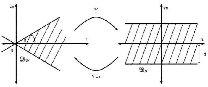
We will now introduce two conformal mappings to transform the eye-shaped and wedge-shaped domains to an infinite strip domain.To do this, we define the function

ν = Φ(z) =ln( z 1−z).

This function Φ provides a conformal transformation of the ”eye-shaped” spatial domain in the z-plane

DE ={z∈C:|arg( z

1−z)|< d},

onto the infinite strip

Ds ={w=u+iv:|v|< d≤

π

2},

(4)

Figure 1. Relationship between the domainsDE and Ds

We define the translated Sinc basis functions

Si(z) =S(i, h)◦Φ(z)≡sinc(

Φ(z)−ih

h ). (3.6)

For the temporal space, we define the function Υ(t) = ln(t) which is a conformal mapping fromDwthe ”wedge-shaped” temporal domain ontoDs, the infinite strip, where:

Dw ={t=r+is:|arg(t)|< d≤

π

2}, this is shown in figure 2.

Figure 2. Relationship between the domains Dw and Ds

The basic functions are derived from the composite translated Sinc functions,

S(j, h)◦Υ(t)≡sinc(Υ(t)−jh

h ). (3.7)

fort∈Dw.

The functionz= Φ−1(v) = _1+eevv is an inverse mapping ofv = Φ(z).

We define the range of Φ−1 on the real line as

(5)

3.1. Interpolation and quadrature rules for approximation:

For problems on a subinterval Γ, of the real line, we employ a conformal map Φ for which Φ(Γ) =R. Suppose d >0 and let Φ be a conformal map of the domainDonto Ds. Then

over a subinterval Γ = Φ−1(R), we apply the following methods of interpolation [22]

f(z)≈

∞

X

k=−∞

f(kh)S(k, h)◦Φ(z). (3.8)

and quadrature:

Z

Γ

f(z)≈h

∞

X

k=−∞

f(zk)/Φ0(zk), (3.9)

The sinc gride pointszk∈(0,1) in DE will be denoted byxi because they are real. For the evenly spaced nodes{ih}∞_i=−∞ on the real line, the image which corresponds to these nodes is denoted by

xi = Φ−1(ih) =

eih

1 +eih, i=±1,±2, . . . and in a same way

tj = Υ−1(jh) =ejh, j =±1,±2, . . . .

The Sinc-Galerkin method actually requires the evaluated derivatives of sinc basis func-tions S(i, h)◦Φ(x) at the sinc nodes, x = xk.The rth derivative of S(i, h)◦Φ(x), with respect to Φ, evaluated at the nodal point xk is denoted by

1

hrδ (r) ik ≡

dr

dΦr[S(i, h)◦Φ(x)]|x=xk . (3.10)

Theorem 3.1. Let Φbe a conformal one-to-one map of the simply connected domainDE onto Ds then

δ_ik(0)= [S(i, h)◦Φ(x)]|x=xk= (

1, k=j;

0, k6=j; (3.11)

δ_ik(1)=h d

dΦ[S(i, h)◦Φ(x)]|x=xk= (

0, k=j; (−1)(k−j)

(k−j) , k6=j;

(3.12)

and

δ_ik(2)=h2 d

2

dΦ2[S(i, h)◦Φ(x)]|x=xk= (_−π2

3 , k=j; −2(−1)(k−j)

(k−j)2 , k6=j.

(3.13)

Proof. See [22].

The expressions in (3.10) for each iand kcan be stored in a matrix

I(p) _{= [}_δ(p)

ik ] forp= 0,1,2:

I(0)= [δ_ik(0)] =



 

1 · · · 0 ..

. . .. ... 0 · · · 1





(6)

I(1)= [δ_ik(1)] =         

0 −1 1₂ · · · (−1)_m−1m−1

1 ...

−1

2 . ..

1 2 ..

. −1

(−1)m

m−1 · · · −1

2 1 0

         , (3.15)

I(2) = [δ(2)_ik ] =

          −π2 3 2 −2 22 · · ·

−2(−1)m−1

(m−1)2

2 ...

−2

22 . ..

−2 22

..

. 2

−2(−1)m−1

(m−1)2 · · ·

−2 22 2

−π2 3           , (3.16)

the above matrices are the m×m(m=M +N + 1) Toeplitz matrices where

−M ≤k≤N, −M ≤i≤N.

If functiong is evaluated at the sinc nodes x=xk for −Mx ≤i≤Nx then the mx×mx square diagonal matrixDmx(g) is written by

Dmx(g) =       

g(x−Mx)

. ..

g(x0) . ..

g(xNx)        . (3.17)

3.2. Parameter selections for the Sinc-Galerkin method.

The matrices that comprise the discrete system in the Sinc-Galerkin method are full matri-ces. More sinc grid points lead to larger matrices and make for an expensive computation. Some cases found in [26] show how to choose an appropriate sinc grid in space and time, and those selections will be used here. If the exact solution satisfies the condition

|u(x, t)| ≤Cxαs+1₂₍₁₋_x₎βs+1₂_tγs+1₂_e−δt_, _(3.18)

for(x, t)∈(0,1)×(0,∞), we should make the following selections

Nx = [|

αs

βs

Mx+ 1|], Mt= [|

αs

γs

Mx+ 1|], Nt= [| 1

hln( αs

δ Mxh) + 1|], (3.19)

where [|.|] denotes the greatest integer operation,h≡hx=ht and

h= ( πd

αsMx

)12. (3.20)

For a given problem with a known real or complex solution, one can determine α, β,γ, andδ using (3.18) where

αs=α− 1

2 and βs=β− 1 2.

Then (3.19) and (3.20) provide the computational parameters. In practice, one sets α =

β = γ = 1 and d = π₂. Then from (3.19) and (3.20), Mx = Nx = Nt and h = ₂√π_M

x,

(7)

interval instead of that given in (3.19).To illustrate the performance of the method, we define kpξk, kqξk and kEξk for reporting error and convergence results between a true solution p(x, t) +iq(x, t) and a Sinc-Galerkin approximate solution ua(x, t) = pa(x, t) +

iqa(x, t) on the sinc gridξ with h=hx =htas

ξ ={(xi, tj) :xi =

eih

1 +eih, tj =e jh_,₋_M

x−1≤i≤Nx+ 1,−Mt≤j≤Nt+ 1}.

3.3. Direct Problem for the Diffusion Equation.

The general form of the diffusion equation is as follow:

P(2)T(x, t)≡Tt(x, t)−a(t)Txx(x, t) =f(x, t), 0< x <1, 0< t <∞, (3.21a)

T(x,0) =φ(x), 0≤x≤1, (3.21b)

T(0, t) =p(t), 0≤t≤ ∞, (3.21c)

T(1, t) =q(t), 0≤t≤ ∞, (3.21d)

φ(x) is a continuous known function, g(t) and q(t) are infinitely differentiable known functions.

We now show the application of the fully Sinc-Galerkin method to solve the direct problem for the diffusion equation. The approximate solution is written as

umx,mt(x, t) =

Nt X

j=−Mt−1

Nx+1 X

i=−Mx−1

uijχi(x)θj(t), (3.22)

where mx = Mx +Nx+ 3 and mt = Mt+Nt+ 2. The basis functions {sij(x, t)} for

−Mx−1≤i≤Nx+ 1,−Mt−1≤j≤Nt are given as the product of basis functions for the appropriate one-dimensional problem. They are given by

sij(x, t)≡[s(i, hx)◦Φ(x)][s(i, ht)◦Υ(t)],

where

Φ(x) =ln( x

1−x), Υ(t) =ln(t). (3.23)

Two linear functions are added to the sinc basis in the spatial dimension

χi(x) =



 

 

1−x, i=−Mx−1,

s(i, h)◦Φ(x), −Mx ≤i≤Nx,

x, i=Nx+ 1,

and one rational function is appended to the temporal base

θj(t) =

(

t+1

t2₊₁, j=−Mt−1,

s(j, h)◦Υ(t), −Mt≤j ≤Nt.

Interpolating the boundary and initial conditions in (3.22) dictates that

umx,mt(0, t) =

Nt X

j=−Mt−1

(8)

umx,mt(1, t) =

Nt X

j=−Mt−1

uNx+1,jθj(t) =q(t),

umx,mt(x,0) =

Nx+1 X

i=−Mx−1

ui,−Mt−1χi(x) =φ(x).

The sinc approximation to (3.22) is defined by

umx,mt(x, t) =

Nt X

j=−Mt

Nx X

i=−Mx

uijsij(x, t) +g∗(t)χ−Mx−1(x)+

q∗(t)χNx+1(x) +φ(x)θ−Mt−1(t),

where

p∗(t) =p(t)−φ(0)θ−Mt−1(t),

q∗(t) =q(t)−φ(1)θ−Mt−1(t),

and the intervals ofiand j confined to −Mx ≤i≤Nx and −Mt≤j ≤Nt, respectively. Somx=Mx+Nx+ 1 and mt=Mt+Nt+ 1.

Define the inner product by

< η, ζ >≡

Z ∞

0

Z 1 0

η(x, t)ζ(x, t)ν(x)ω(t)dxdt,

where the productν(x)ω(t) plays the role of a weight function. Assume that the product is given by

ν(x)ω(t) =

√

Υ0 Φ0 , where

ω(t) =√Υ0_, _ν₍_x_{) =} 1 Φ0.

Sincep∗(t) and q∗(t) are known functions, the orthogonalization of the residual

< P(2)umx,mt−f, skl>= 0,

for−Mx ≤k≤Nx,−Mt≤l≤Nt may be written

< P(2)uh−f∗, skl>= 0, (3.24) where the homogeneous part of the approximate solution is given by

uh(x, t) = Nt X

j=−Mt

Nx X

i=−Mx

uijsij(x, t),

f∗ is also given by

f∗(x, t) =f(x, t)−P(2)[p∗(t)χ−Mx−1(x) +q

∗₍_t₎_χ

(9)

3.4. Discrete System Assembly.

Now we want to discrete the system of (3.24):

< ut, skl>−< a(t)uxx, skl>−< f∗, skl>= 0. The inner product with sinc basis elements is given by

< ut, skl>=

Z ∞

0

Z 1

0

utsklν(x)ω(t)dxdt.

This expression contains derivative of u with respect tot. We can remove derivative from the dependent variable u by integrating by parts, once doing this in t. We obtain the following term

BT1 −

Z ∞

0

Z 1

0

uh(x, t)[s(k, hx)◦Φ(x)]ν(x)([s(l, ht)◦Υ(t)]ω(t))0dxdt,

where the boundary term

BT1 =

Z 1

0

[s(k, hx)◦Φ(x)]ν(x)([s(l, ht)◦Υ(t)]ω(t)uh(x, t))|∞_t=0 dx= 0.

If we do the similar calculations for< a(t)uxx, skl>, then we have

< a(t)uxx, skl>=

Z ∞

0

Z 1

0

a(t)uxxsklν(x)ω(t)dxdt.

This expression contains the derivatives of the dependant variable u, twice inx. We can similarly removeuxx by integrating by parts, as follows:

BT2−

Z ∞

0

Z 1

0

a(t)uh(x, t)[s(l, ht)◦Υ(t)]ω(t)([s(k, hx)◦Φ(x)]ν(x))00dxdt,

where the boundary term

BT2 =

Z ∞

0

a(t)[s(l, ht)◦Υ(t)]ω(t)([s(k, hx)◦Φ(x)]ν(x))0uh(x, t))|1x=0 dt

−

Z ∞

0

a(t)[s(l, ht)◦Υ(t)]ω(t)([s(k, hx)◦Φ(x)]ν(x)ux(x, t))|1x=0dt = 0.

Remove the derivatives from the dependent variable u by integrating by parts; twice in x and once in t, to arrive at the identity

Z ∞

0

Z 1

0

uh(x, t)(−

∂ ∂t−

∂2

∂x2)(sk(x)sl(t)ν(x)ω(t))dxdt=

Z ∞

0

Z 1

0

f∗sk(x)sl(t)ν(x)ω(t)dxdt.

We apply the quadrature rule [22] to the iterated integrals and delete the error terms.We also replaceuh(x, t) by uij and dividing by hxht. Hence, we obtain the following discrete sinc system:

a(tl) ω(tl) Υ0₍_t

l) Nx X

−Mx

[− 1

h2 x

δ_ki(2)Φ0(xi)ν(xi)− 1

hx

δ_ki(1)(Φ

00₍_x_i)_ν₍_x_i) Φ0₍_x

i)

+2ν0(xi))−δ_ki(0)ν

00₍_x_i)

Φ0₍_x_i)]uil (3.26)

+ν(xk) Φ0₍_x

k) Nt X

j=−Mt

[−1

ht

δ_lj(1)ω(tj) +δ(0)lj

ω0(tj) Υ0₍_t

j)

(10)

= f ∗₍_x

k, tl)ν(xk)ω(tl)

Φ0(xk)Υ0(tl) . (3.28) This system is identical to the system generated by orthogonalizing the residual via < p(2)uh−f∗, skl>= 0. We apply the notation of section 2 and obtain the following matrix form

[−1

h2 x

I_m(2)_xD(Φ0ν)− 1

hx

I_m(1)_xD(Φ 00_ν

Φ0 + 2ν

0₎₋_I(0) mxD(

ν00

Φ0)]U

(2)_D₍a ω Υ0 )

+D(ν Φ0)U

(2)_[−1

ht

I_m(1)_tD(ω) +I_m(0)_tD(ω 0

Υ0)]

=D(ν Φ0)F

(2)_D₍ω Υ0),

premultiplying byD(Φ0) and postmultiplying byD(Υ0) yields the equivalent system

D(Φ0)[−1

h2 x

I_m(2)_xD(Φ0ν)− 1

hx

I_m(1)_xD(Φ 00_ν

Φ0 + 2ν 0

)−I_m(0)_xD(ν 00

Φ0)]U

(2)_D₍_{a ω}₎

+D(ν)U(2)[−1

ht

I_m(1)_tD(ω) +I_m(0)_tD(ω 0

Υ0)] T_D_(Υ0

)

=D(ν)F(2)D(ω).

It is helpful to single out the portion of the coefficient matrix in this system that corre-sponds to the second derivative. This is defined by

A(v)≡ −1

h2 x

I_m(2)_x− 1

hx

I_m(1)_xD( Φ 00

(Φ0₎2 + 2ν0

Φ0_ν)−D(

ν00

(Φ0₎2_ν), (3.29)

B(

√

Υ0) = −1

ht

I_m(1)_t −D( ω 0

ωΥ0) =

−1

ht

I_m(1)_t +D(1

2), (3.30) the second equality follows from _ωΥω00 = Υ

00

2(Υ0₎2 ≡

−1

2 ,where Υ =ln(t).

The representation of the system is simplified upon recalling the definition of the matrix

A(ν) and B(√Υ0_{) in (3.29) and (3.30), respectively.} Finally we reach to the form as follow:

Axν

(2)

D(a(t)) +ν(2)B_tT =G(2), (3.31) where

Ax =D(Φ0)A(v)D(Φ0) =D(Φ0)[

−1

h I

(2)₊_D₍ −1 (Φ0₎3₂(

1

√

Φ0)

00_)]_D_(Φ0₎_,

Bt=D((Υ0)

1 2)[−1

hI

(1)₊_D₍1

2)]D((Υ 0₎1

2),

ν(2) =D(ν)U(2)=D((Φ0)−21)U(2), G(2) =D(ν)F(2)=D((Φ0)−21)F(2).

In the latter, the matrixF(2) is now the matrix of point evaluations off∗ in (3.25). We discretize the system and find it’s matrix form and transform obtained equation to follow equation by using theorem A.33 in [22];

AΘ =B,

(11)

Thus the linear system corresponding to the sinc coefficientuij can be expressed as

AΘ =B. (3.32)

The Matrix Ais ill-conditioned. On the other hand, asg(t) is affected by measurement errors, the estimate of Θ by (3.32) will be unstable so that the Tikhonov regularization method must be used to control this measurement errors. The Tikhonov regularized solution ( [27], [28], [29], and [30]) to the system of linear algebraic equation (3.32) is given by

zα(Θ) =kAΘ−Bk22+αkR(s)Θk22.

On the case of thezeroth -, first-, and second-order Tikhonov regularization method the matrixR(s), fors= 0,1,2,is given by, see e.g. [31]:

R(0) =IM1×M1 ∈R

M1×M1_,

R(1) =



     

−1 1 . . . 0 0 0 0 −1 1 . . . 0 0

..

. ... ... ... ... ... 0 0 . . . −1 1 0 0 0 . . . 0 −1 1



     

∈_R(M1−1)×M1_,

R(2) =



     

1 −2 1 0 . . . 0 0 0 1 −2 1 0 . . . 0

..

. ... ... ... ... ... ... 0 0 . . . 1 −2 1 0 0 0 . . . 0 1 −2 1



     

∈_R(M1−2)×M1_,

whereM1= (γ+ 1)×(ι+ 1).

Therefore, we obtain the Tikhonov regularized solution of the regularized equation as

Θα =ATA+α(R(s))TR(s)−1ATB.

In our computation, we use the GCV scheme to determine a suitable value ofα( [32], [33] and [34]).

Theorem 3.2. For each fixedt, letF(x, t)∈B(DE)andh >0. LetΦandΥbe one-to-one conformal maps of the domainsDE andDw ontoDs, respectively. Let xi = Φ−1(ihx), tj = Υ−1(jht) and Γx= Φ−1(R),Γt= Υ−1(R).Assume there are positive constantsαx, βx and

Cx(t) so that

| F(x, t)

Φ0(x) |≤Cx(t)

(

exp(−αx |Φ(x)|, x∈Γ(x)a ,

exp(−βx |Φ(x)|, x∈Γ (x) b , where

Γ(x)_a ≡ {x∈Γx: Φ(x) =u∈(−∞,0)}, Γ(x)_b ≡ {x∈Γx: Φ(x) =u∈(0,∞)}. Also for each fixed x, letF(x, t) ∈ B(Dw)and assume there are positive constants αt, βt andCt(x) so that

| F(x, t)

Υ0₍_x₎ |≤Ct(x)

(

exp(−αt|Υ(t)|, x∈Γ(t)a ,

exp(−βt|Υ(t)|, x∈Γ(t)_b , where

Γ(t)_a ≡ {t∈Γt: Υ(t) =u∈(−∞,0)}, Γ (t)

(12)

Then the sinc trapezoidal quadrature rule is

Z

Γt Z

Γx

F(x, t)dxdt=hxht Nx X

i=−Mx

Nt X

j=−Mt

F(x, t) Φ0₍_x

i)Υ0(tj)

+O(exp(−αxMxhx))

+O(exp(−βxNxhx)) +O(exp(

−2πd hx

)) +O(exp(−αtMtht)) +O(exp(−βtNtht))

+O(exp(−2πd

ht )).

Hence, make the selections

Nx= [|

αx

βx

Mx+ 1|], Mt= [|

αx

αt

Mx+ 1|], Nt= [|

αx

βt

Mx+ 1|]

where h≡hx =ht and

h=

r

2πd αxMx

and the exponential order of the sinc trapezoidal quadrature rule is O(e−(

√

2πdαxMx)

1 2

).

Corollary.An important special case housed in the previous theorem occurs when the double integrand has the formG(x, t)S(p, hx)◦Φ(x)S(q, ht)◦Υ(t).Due to the interpolation

S(p, hx)◦Φ(x) =S(p, hx)(ihx) =δ(0)_ip and S(q, ht)◦Υ(t) =S(q, ht)(jht) =δ_jq(0),

the sinc quadrature rule is a weighted point evaluation to the order of the method

Z

Γt Z

Γx

G(x, t)S(p, hx)◦Φ(x)S(q, ht)◦Υ(t)dxdt=hxht

G(xp, tq) Φ0₍_x

p)Υ0(tq) +O(exp(−2πd_h

x )) +O(exp(

−2πd ht )).

Proof. See [26].

4. Genetic algorithm

Genetic algorithms, primarily developed by Holland [35], have been successfully applied to various optimization problems. It is essentially a searching method based on the Dar-winian principles of biological evolution. Genetic algorithm is a stochastic optimization algorithm which employs a population of chromosomes; each of them represents a possible solution. By applying genetic operators, each successive incremental improvement in a chromosome becomes the basis for the next generation. The process continues until the desired number of generations has been completed or the predefined fitness value has been reached.

Typically binary coding is used in classic genetic algorithm, where each solution is en-coded as a chromosome of binary digits. Each member of the population represents an encoded solution in the classic genetic algorithm. For many problems, this kind of coding is not natural. The genetic algorithm used in this work is not a classic genetic algorithm. Instead, the application of genetic algorithm to this discrete-time optimal control problem is called a real-valued genetic algorithm(RVGA). The continuous function is discrete for numerical computation and simulated by a chromosome. The value of each gene is a real number and indicates the heat generation at each time step [36].

The procedure of a RVGA is as follows:

(13)

Step 2. Evaluate the fitness of each chromosome in the population.

Step 3. Select chromosomes, based on the fitness function, for recombination. Step 4. Recombine pairs of parents to generate new chromosomes.

Step 5. Mutate the resulting new chromosomes. Step 6. Evaluate the fitnesses of new chromosomes. Step 7. Update population.

Step 8. Repeat Step 3 to Step 7, until the fitness function is convergent or less than a predefined value.

5. A modified RVGA to determine a(t)

In this paper, we have used a modified RVGA to determine a(t). We guess a(t) by

a(t) =a×(b+c×x+d×x 2

e+f×x+g×x2) equation. Wherea,b,c,d,e,f andgare coefficients, that the modified RVGA must find them. In the modified RVGA, chromosomes are encoded as real-valued vectors. J-th element of each chromosome is j-th coefficient. We consider each element of chromosomes as a gene. Thatgp,j is j-th gene of chromosome ofp. For finding optimal solution of a(t), the Equation (2.2) should be minimum. For this purpose, we consider Equation (2.2) as fitness function and calculate simulatedsby solving nonlinear direct heat parabolic problem by sinc-galerkin method for each chromosome. At the end of algorithm, the chromosome by lowest fitness is the best solution of a(t). To improve the performance of RVGA, we added a new step to algorithm after ”mutation” operator, for modifying new chromosomes at each iteration.

The procedure of a modified RVGA is as follows:

Step 1. Generate at random an initial population of chromosomes. Step 2. Evaluate the fitness of each chromosome in the population. Step 3. Select some chromosomes as parents by tournament selection.

Step 4. For generating pair of new chromosomes, pair of parents crossover together as follow:

gch1,j =α×gp1,j+ (1−α)×gp2,j, j= 1,2,3, ..., M,

gch2,j=β×gp1,j+ (1−β)×gp2,j, j= 1,2,3, ..., M.

Wherep1 illustrates first parent,p2 illustrates second parent,ch1 illustrates first new chromosome, ch2 illustrates second new chromosome, α and β are random numbers in [−0.25,1.25].

Step 5. For applying ”Mutation” operation on new chromosomes, selecting a gene of each new chromosome randomly and each element of genes adding by random number. Step 6. Finding the first best gene between new chromosomes and copy that gene to first gene of all chromosomes. Then finding the second best gene between new chromosomes and copy that gene to second gene of all chromosomes. Continue this procedure for all genes. Now all new chromosomes are same. For generating new hopeful chromosomes, genes of second to end chromosomes replace by genes of first chromosome adding by random small values.

Step 7. Evaluate the fitness of new chromosomes. Step 8. Update the population.

(14)

6. Numerical results

We are going to demonstrate numerically, some of results for the unknown function

a(t) in the IDP (2.1). The aim of this section is to illustrate the applicability of the present method described in Section 5 for solving IDP. As expected the IDP is ill-posed and therefore it is necessary to investigate the stability of the present method by giving some test problems.

In this section, we have two examples, for 0< x <1,0< t <1. Our first example is

Example 6.1.

T(x,0) = sin(πx), 0≤x≤1, (6.1b)

T(0, t) = 0, 0≤t≤tM, (6.1c)

T(1, t) =e−π2t2(sin(π)), 0≤t≤tM, (6.1d)

s(tj) =U(0.9, tj) +σR, j = 1,2,3,· · · ,9, (6.1e)

where tj’s are the sinc times nodes, the exact a(t) is 2t and the exact T(x, t) is

e−π2t2(sin(πx)).

The second example is

Example 6.2.

T(x,0) = 1 3e

−x_, ₀_≤_x_≤₁_, _(6.2b)

T(0, t) = t 2_{+ 1}

3 , 0≤t≤tM, (6.2c)

T(1, t) =e−1(t 2_{+ 1}

3 ), 0≤t≤tM, (6.2d)

s(tj) =U(0.9, tj) +σR, j = 1,2,3,· · · ,9, (6.2e)

where, tj’s are the sinc times nodes, the exact value ofa(t) is 2t

t2_{+ 1} and the exact value ofT(x, t) ise−x(t

2_{+ 1} 3 ).

The experimental data s(tj) (measured temperatures) are obtained from the exact so-lution of the direct problem by adding a random perturbation error to the exact soso-lution of the direct diffusion problem in order to generate noisy data, whereσ= 0.001 and R is a random value in (0,1).

(15)

second source of error is the variance due to the amplification of measurement errors (sto-chastic error). The global effect of deterministic and sto(sto-chastic errors is considered in the mean squared error or total error, [12].

S=

h 1

(N −1) N

X

i=1

(abi−ai)

2i

1 2

, (6.3)

where N is the total number of estimated values, a_bi is calculated values from guessed a(t) andai is exact values of a(t).

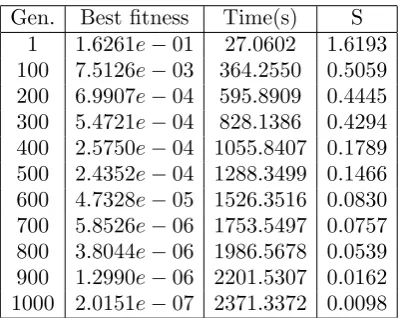
In our examples, here, a population of 20 chromosomes of 7 genes(a,b,c,· · ·,g) is used as the initial guess to obtain for numerical results of modified RVGA. Table 1 presents the results for 1 to 1000 generations for the first example and Table 2 presents the results for 1 to 1000 generations for the second example. Note thatS calculated by 10 total number of points.

Gen. Best fitness Time(s) S 1 4.1270e−02 14.8147 1.2058 100 8.1576e−04 244.9134 0.9575 200 5.9278e−04 458.4853 0.8002 300 4.2176e−04 702.1418 0.6557 400 6.0035e−05 928.8491 0.1548 500 7.5774e−05 1149.7431 0.2227 600 5.8481e−06 1382.1371 0.0482 700 7.6551e−06 1614.9502 0.0646 800 1.7093e−06 1817.3170 0.0175 900 3.1832e−07 2039.2769 0.0045 1000 2.4076e−07 2260.1846 0.0018

Table 1. The results of modified RVGA for a population of 20 chromo-somes of 7 genes for 1 to 1000 generations for the first example.

Gen. Best fitness Time(s) S 1 1.6261e−01 27.0602 1.6193 100 7.5126e−03 364.2550 0.5059 200 6.9907e−04 595.8909 0.4445 300 5.4721e−04 828.1386 0.4294 400 2.5750e−04 1055.8407 0.1789 500 2.4352e−04 1288.3499 0.1466 600 4.7328e−05 1526.3516 0.0830 700 5.8526e−06 1753.5497 0.0757 800 3.8044e−06 1986.5678 0.0539 900 1.2990e−06 2201.5307 0.0162 1000 2.0151e−07 2371.3372 0.0098

Table 2. The results of modified RVGA for a population of 20 chromo-somes of 7 genes for 1 to 1000 generations for the second example.

(16)

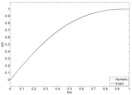
Figure 3. The exact and numerica(t) for the first example by implement-ing modified RVGA for 1000 generation.

Figure 4. The exact and numerica(t) for the second example by imple-menting modified RVGA for 1000 generation.

7. Conclusion

(17)

(1) The present study successfully applies the numerical method to the inverse diffu-sion problem (IDP).

(2) To solve the IDP by using the genetic algorithm, the unknown function will be guessed and we don’t need the regularization. This will improve the execution time.

(3) To solve the direct diffusion problem, we used the Sinc-Galerkin method. There-fore, we obtain the solution of direct problem in a more extensive time range. In fact, the solutions are obtained in the whole domain. Furthermore, this method improves the execution time for solving direct diffusion problem.

(4) Results show that a good estimation can be obtained by combining the genetic algorithm and the Sinc-Galerkin method within a CPU with clock speed 2.7 GHz.

References

[1] Cannon,J.R. and Van de Hoek,J., (1982), The one phase stefan problem subject to energy, J. Math. Anal. Appl., 86, pp.281-292.

[2] Cannon,J.R., Eteva,S.P., and Van de Hoek,J., (1987), A Galerkin procedure for the diffusion equation subject to the specification of mass, SIAM J. Numer. Anal., 24, pp.499-515.

[3] Cannon,J.R., (1963), The solution of the heat equation subject to the specification of energy, Quart. Appl. Math., 21, pp.155-160.

[4] Capasso,V. and Kunisch,K., (1988), A reaction-diffusion system arising in modeling manevironment diseases, Quart. Appl. Math., 46, pp.431-450.

[5] Shidfar,A., Pourgholi,R., and Ebrahimi,M., (2006), A numerical method for solving of a nonlinear inverse diffusion problem, Comput. Math. Appl., 52, pp.1021-1030.

[6] Dehghan,M., (2001), An inverse problem of finding a source parameter in a semilinear parabolic equation, Appl. Math. Model., 25, pp.743-754.

[7] Dehghan,M., (2002), Numerical techniques for a parabolic equation subject to an overspecified bound-ary condition, Appl. Math. Comput. 132, pp.299-313.

[8] Dehghan,M., (2003), Numerical solution of one-dimensional parabolic inverse problem, Appl. Math. Comput., 136, pp.333-344.

[9] Tatari,M. and Dehghan,M., (2007), Identifying a control function in parabolic partial differential equations from overspecified boundary data, Computers and Mathematics with Applications, 53, pp.1933-1942.

[10] Beck,J.V., Blackwell,B., and St.Clair,C.R., (1985), Inverse Heat Conduction: IllPosed Problems, Wiley-Interscience, NewYork.

[11] Beck,J.V. and Murio,D.C., (1986), Combined function specification-regularization procedure for solu-tion of inverse heat condisolu-tion problem, AIAA J., 24, pp.180-185.

[12] Cabeza,J.M.G., Garcia,J.A.M., and Rodriguez,A.C., (2005), A Sequential Algorithm of Inverse Heat Conduction Problems Using Singular Value Decomposition, International Journal of Thermal Sciences, 44, pp.235-244.

[13] Molhem,H. and Pourgholi,R., (2008), A numerical algorithm for solving a one-dimensional inverse heat conduction problem, Journal of Mathematics and Statistics, 4(1), pp.60-63.

[14] Pourgholi,R., Azizi,N., Gasimov,Y.S., Aliev,F., and Khalafi,H.K., (2009), Removal of Numerical Insta-bility in the Solution of an Inverse Heat Conduction Problem, Communications in Nonlinear Science and Numerical Simulation, 14(6), pp.2664-2669.

[15] Pourgholi,R. and Rostamian,M., (2010), A numerical technique for solving IHCPs using Tikhonov regularization method, Applied Mathematical Modelling, 34(8), pp.2102-2110.

[16] Pourgholi,R., Rostamian,M., and Emamjome,M.,(2010), A numerical method for solving a nonlinear inverse parabolic problem, Inverse Problems in Science and Engineering, 18(8), pp.1151-1164. [17] Tadi,M., (1997), Inverse Heat Conduction Based on Boundary Measurement, Inverse Problems, 13,

pp.1585-1605.

[18] Shidfar,A., Zolfaghari,R., and Damirchi,J., (2009), Application of Sinc-collocation method for solving an inverse problem,Journal of computational and Applied Mathematics, 233, pp.545-554.

(18)

[20] Pourgholi,R., Dana,H., and Tabasi,S.H., (2014), Solving an inverse heat conduction problem using ge-netic algorithm: Sequential and multi-core parallelization approach, Applied Mathematical Modelling, Volume 38, Issues 78.

[21] Pourgholi,R., Molai,A.A., and Houlari,T., (2013), Resolution of an inverse parabolic problem using Sinc-Galerkin method, TWMS J. App. Eng. Math.,V2(3), pp.160-181.

[22] Lund,J. and Bowers,K., (1991), Sinc Methods for Quadrature and Differential Equations, Siam, Philadelphia, PA.

[23] Stenger,F., (1979), A Sinc-Galerkin method of solution of boundary-value problems, Math. Comp., 33, pp.85-109.

[24] Whittaker,E.T., (1915), On the functions which are represented by the expansions of the interpolation theory, Proc. Roy. Soc. Edinburg, 35, pp.181-194.

[25] Whittaker,J.M., (1935), Interpolation Function Theory, in: Cambridge Tracts in Mathematics and Mathematical Physics, Vol.33, Cambridge University Press, London.

[26] Koonprasert,S. and Bowers,K., (2004), The Fully Sinc-Galerkin Method for Time-Dependent Bound-ary Conditions, Numerical Method for Partial Differential Equations, 20(4), pp.494-526.

[27] Hansen,P.C., (1992), Analysis of discrete ill-posed problems by means of the L-curve, SIAM Rev., 34, pp.561-80.

[28] Lawson,C.L. and Hanson,R.J., (1995), Solving Least Squares Problems, Philadelphia, PA:SIAM. [29] Tikhonov,A.N. and Arsenin,V.Y., (1977), On the solution of Ill-posed problems, New York, Wiley. [30] Tikhonov,A.N., and Arsenin,V.Y., (1977), Solution of Ill-Posed Problems, V.H.Winston and Sons,

Washington, DC.

[31] Martin,L., Elliott,L., Heggs,P.J., Ingham,D.B., Lesnic,D., and Wen,X., (2006), Dual Reciprocity Boundary Element Method Solution of the Cauchy Problem for Helmholtz-type Equations with Vari-able Coefficients, Journal of sound and vibration, 297, pp.89-105.

[32] Elden,L., (1984), A Note on the Computation of the Generalized Cross-validation Function for Ill-conditioned Least Squares Problems, BIT, 24, pp.467-472

[33] Golub,G.H., Heath,M., and Wahba,G., (1979), Generalized Cross-validation as a Method for Choosing a Good Ridge Parameter, Technometrics, 21(2), pp.215-223.

[34] Wahba,G., (1990), Spline Models for Observational Data, CBMS-NSF Regional Conference Series in Applied Mathematics, Vol.59, SIAM, Philadelphia.

[35] Holland,J.H., (1975), Adaptation in Natural and Artificial System, University of Michigan Press, Ann Arbor.

[36] Liu,F-B., (2008), A modified genetic algorithm for solving the inverse heat transfer problem of esti-mating plan heat source, International Journal of Heat and Mass Transfer, 51, pp.3745-3752.

Reza Pourgholi, for the photograph and short biography, see TWMS J. Appl. and Eng. Math., V.2, No.2, 2012.

Hassan Dana Mazraeh is a lecturer at Damghan University, School of Math-ematics and Computer Science, Iran. His areas of research are evolution-ary computing, numerical analysis, and scientific computing. Web address: http://faculty.du.ac.ir/dana/.