The Effect of Lateral Boundary Conditions on
Results of One-Way Nested Ocean Regional
Circulation Model
Van Sy Pham
1*and Jin Hwan Hwang
1†1Seoul National University, 1 Gwanak-ro, Gwanak-gu, 151-744, Seoul, Korea
Abstract
This research evaluated two main sources of impact on the results of the ocean regional circulation model (ORCMs) during downscaling and nesting the results from the ocean global circulation model (OGCMs). Representative two sources should be the spatial resolution difference between driving and driven data, and the frequency for up-dating LBCs. The Big-Brother method investigated the effect of them on the results of the ORCMs separately. The results showed that the lateral boundary conditions (LBCs) potentially degraded the results of ORCMs. The errors developed at the boundaries propagate slowly into the center of the nested domain as time passes. The simulation results of the ORCMs significantly depend not only on spatial resolution but also on the frequency for updating the lateral boundary conditions. The ratio resolution of spatial resolution between driving data and driven model can be up to 3 and the updating frequency of the LBCs can be up to every 6 hours per day.
1
Introduction
The oceanic regional circulation model (ORCMs) is an efficiency tool to dynamically downscale the low temporal and spatial resolution of global model to obtain greater resolution on a regional scale ( (Voronkov, EasyChair conference system, 2004) Li et al. 2012; Herbert et al. 2014; Pham et al. 2016) The ORCM needs local information such as wind forcing, heat radiation, and precipitation for the initial and boundary conditions at the sea surface. In addition, the ORCMs also requires information on large-scale oceanic fields that vary with time, such as momentum, sea surface height, temperature and salinity fluxes through the lateral boundary conditions (LBCs) to calculate local currents and tracers (Marchsiello et al. 2001; Mcdoland. 1999). These kinds of models are known as one-way nested ORCMs. However, the procedures employed while downscaling and nesting this
*
Volume 3, 2018, Pages 1631–1638
larger scale information into smaller scale models, produce unwanted errors (Warner et al. 1997). Representative two issues affecting the results of the ORCMs should be spatial resolution different between nesting data and nested model, and the frequency for up-dating the LBCs. In this research, the characteristic of these issues are exposed, and their effects on ORCMs are performed. The main objectives of this research are to answer the questions as follows:
• How does the spatial resolution of LBCs impact to the results of the ORCMs?
• How does the updating frequency of LBCs affect to the ORCMs results?
2
Study method
2.1
The Big-Brother Experiment
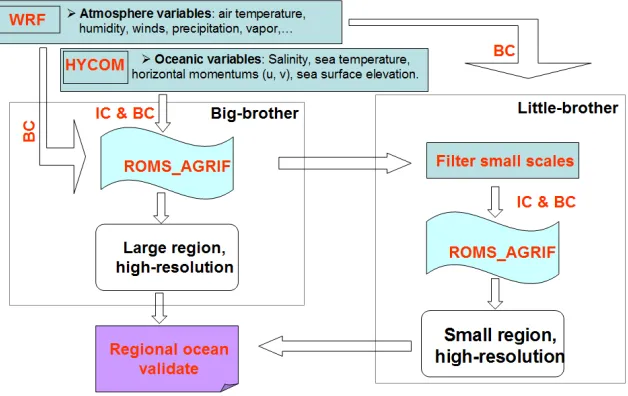
We employ Big-Brother Experiment (BBE) developed with purpose of examining the downscaling ability of nested regional climate models (RCMs) (Denis et al. 2002). Figure 1 shows schematic diagram of the BBE. The BBE firstly simulated high resolution limited area model. It is called as Big-Brother in the large domain. The simulation results of the Big-Brother, which filtered the short scales, are used to drive the embedded domain of Big-Brother. This embedded domain is called as Little-Brother. It is consisting of high-resolution grid as same as the Big-Brother. This experimental method is considered as a “perfect-prognosis” approach and further results in no model errors and observation limitation. Moreover, the both large and small scaled diagnostic values of the Little-Brother can easily compare to the Big-Brother because of the same high resolution. The differences between the Big-Brother and Little-Brother can be regarded as errors resulted from the nesting and downscaling techniques. (See Pham et al. 2016; Denis et al. 2002 for more details).
2.2
The Model set-up
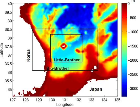
In this research, our study area is the East Sea of Korea. Both Big-Brother and Little-Brother have spatial resolution of 3 km × 3 km grid cells , sketching from 128.50οE to 133.50οE in longitude and
36.10οN to 38.51οN in latitude. The Little-Brother is the small domain, has the same spatial resolution
and embedded in the Big-brother domain. The domain size of the Little-Brother ranges from 129.90οE
to 132.30οE in longitude and 36.58οN to 38.19οN in latitude as shown in Figure 2. Both domains have
30 vertical layers of S-grid.
The simulation time is from September 1st to September 30th, 2011 (30 days). The time step of integration used in both the Big-Brother and Little-Brother were 10 minutes. The oceanic variables were downloaded from the HYbird Coordinate Ocean Model (HYCOM) Global Hindcast. They have spatial resolution at 1/12ο× 1/12ο (~ 9 km) 12 hours output frequency. The regional ocean circulation
model used in this research was ROMS_AGRIF which is a version of Regional Ocean Modeling System (ROMS) using the adaptive grid refinement in Fortran (AGRIF) nesting procedure (Cambon et al. 2014; Hedstrom et al. 2009). The open boundary condition (OBC) applied in the research is radiation boundary condition with an additional nudging term adding to the radiation boundary equation (Marchsiello et al. 2001). This OBC works well for waves propagating not only normal to the boundary, but also approaching the boundary at an angle. Also, it can prevent substantial drifts while avoiding over specification problems during the outward propagation, and produces a data-shock problem during inward propagation. The initial conditions were provided only one time at the beginning of nearly one month integration. The initial conditions can be considered as perfect ones because the same resolution was used in the Big-Brother and Little-Brother to avoid interpolation errors which are not further perturbed.
dataset corresponding to 3km resolution of Little-brother. Five updating frequencies implemented are U1, U6, U12, U16 and U24, corresponding to 1, 6, 12, 16, 24 every hours per day of update intervals, respectively as shown in the Table 1.
To mimic the resolution of ocean global circulation models at resolution at 9 × 9 km, all wavelengths smaller than 18 km of both oceanic diagnostic variables of Big-Brother and atmospheric simulation variables of the WRF are filtered before applying to the Little-Brother. The method filtering the small scale is Discrete Cosine Transform (DCT). It has an efficient capacity to treat aperiodic fields by taking a mirror image of the original function for analyzed periodic fields prior to the application of the discrete Fourier transform. (See Denis et al. 2002) for more details on DCT). The resolution jump between the Big-Brother and Little-Brother is considered as 3. The resolution jump is spatial resolution difference between the driver and the nested model Denis et al. 2002). It is calculated by dividing the filtered wavelengths of Big-Brother by the shortest resolvable wavelength of the Little-Brother. For instance, the filter wavelengths of the Big-Brother is 18 km, the shortest resolvable wavelength of the Little-Brother is 2×3km. Therefore, the resolution jump is 3 (18km/(2×3 km).
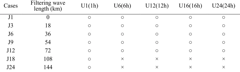
Cases Filtering wave length (km) U1(1h) U6(6h) U12(12h) U16(16h) U24(24h)
J1 0 ○ ○ ○ ○ ○
J3 18 ○ ○ ○ ○ ○
J6 36 ○ ○ ○ ○ ○
J9 54 ○ ○ ○ ○ ○
J12 72 ○ ○ ○ ○ ○
J18 108 ○ × × × ×
J24 144 ○ × × × ×
Table 1: The list of performed experiments. The ○s cells are simulated and the ×s cells were skipped
3
Results
The errors driven by LBCs might affect significantly the nested model results. They are unique and unavoidable aspects of the downscaling process (Mcdoland, 1999; Warner et al. 1997; Denis et al. 2002). As time pass, such errors propagate into the inner domain and as a result they degrade the solution of the nested model. These effects caused by the ‘way of the LBC formulation’ and the ‘temporal and spatial resolution different between driving data and driven model’. Such effects are separately evaluated below.
3.1
Effects of the way of LBCs formulation
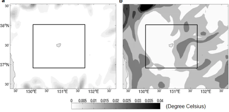
To addressed how the errors affected by the way of LBCs formulation, the jump ratio was set at 1 (J1), the time interval of the Little-Brothers and the update frequency of the LBCs were set up at 10 minutes. The targeted Little-Brother has domain size of 306 × 246km. The RMS values of the different between Big-Brother and targeted Little-Brother from the first to thirtieth day were calculate after depth-averaging the temperature of the two domains. The errors of temperature (black or gray areas in Figure 3 (a)) just occurred along the boundaries. Their value decreased toward center. There is no error inside the targeted area shown by the black rectangular line in the Figure 3(a). After 30 days of simulation, the errors transmit into the targeted area Figure 3 (b).
3.2
Spatial resolution of the LBCs affect on the results of ORCMs
The impact of the LBCs spatial resolution on the result of ORCMs is experimented with the fixed period of updating frequency.The temporal update frequency must equate to interval of driven model (10 minutes). However, there are almost no differences of solutions with the update frequency of LBCs smaller than 1 hour in our experiments (not shown here). Therefore, we select 1 hour of LBC update frequency for a convenient.
From the results of experiment with seven different resolutions and five different update frequencies of LBCs, they show that the resolution jump quite affects on the salinity. In general, the quality of salinity field better as spatial resolution jump become smaller. For example, as the jump ratio increase from J6 to J24, correlation coefficient decrease. However, at the spatial resolution ratio smaller than 6, the quality of salinity field is not alone determined by spatial resolution jump, and J3 become better than J1.
1-2 psu over 34 psu. However, when the spatial resolution ratio smaller than 6, the temperature field is also not controlled by spatial resolution jump since the J3 and J6 perform better than J12. The acceptable ratio of spatial resolution can be chosen at J3 with a correlation coefficient of both temperature and salinity greater than 0.91. Opposing to salinity and temperature fields, the z-vorticity fields express better as the spatial resolutions increase. The acceptable resolution jump can also get up to J3 with approximately 0.97 of correlation coefficient.
3.3
The temporal update of the results of the ORCMs
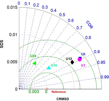
Different with the spatial analysis, the qualities of the temperature fields do not always perform better when the updating times become shorter (Fig. 4). For example, the case of U6 which means that updated at every 6 hours has higher correlation coefficient and less CRMSD comparing to U1 which is rapid updating case. However, the different values of them are quite small. The difference of correlation coefficient between two case is only 0.05, and CRMSD is 0.006 0. The result of salinity is quite similar to temperature. In contrast to temperature and salinity, vorticity fields is quite sensitive to the change of temporal update of the LBCs. The quality of voticity reproduction is better with shorter updating intervals. The acceptable temporal update of the LBCs can be chosen at U6 since correlation coefficient of all diagnostic variables including temperature, salinity and vorticity are greater than 0.9.
In the previous section, the resolution jump J3 and updating frequency at U6 are selected. Therefore, the column at U6 and the line at the J3 are checked to figure out whether their resolution at intersection is satisfied. The results show the good agreement for the pair J3 and U6 since the correlation coefficient of all fields are higher than 0.87.
4
Summary and conclusions
Qualifying the errors resulted from the diverse sources during dynamic downscaling the lower resolved information from the global model into ORCM with higher resolutions and fine time steps is really a challenge. Such errors affect the results from the ORCMs in the different levels of the temporal updating of simulation, the location of appearance, the natural condition of research areas and the diagnostic variables (Pham et al. 2016; Warner et al. 1997; Denis et al. 2002) including temperature, salinity and vorticity. One source of error can associate with others to worse the ORCMs results and once error sources are interconnected (Warner et al. 1997), then it makes difficult to assess each contribution of error on the results of ORCMs. The present research applying Big Brother Experiments characterized these error sources and assessed those effects on ORCMs results as separately as possible. Therefore, it enables to quantitatively assess the contribution of each error source to the nesting and downscaling using the ORCMs. From the results discussed in the previous sections, let us summary the research as follow:
• The simulation results of the ORCMs significantly depend on the spatial resolution of the LBCs. The interpolation of the lateral boundaries can cause the error to degrade the accuracy for prediction. In general, lower spatial resolutions from the OGCMs results increase errors along the boundaries. The ratio of the spatial resolutions between original data and nested model can be up to 3, which is resolved at 3 km for the grid size of the ORCMs.
• The solution of the ORCMs also depends on the temporal resolution of the LBCs. However, although the decreasing the ratio of spatial resolution jump increase the quality of production, the shorter updating intervals do no guarantee higher performance of results of the ORCMs. The updating frequency of the LBCs does not greatly affect temperature and salinity but does for vorticity. The recommended updating interval of the LBCs can be every 6 hoursof LBCs affect to the ORCMs results.
Our research only works with a kind of numerical model, resolution of inner domain and region which are play important role in the simulating results. Since the different resolution can differently develop small scale features. In addition, the resolution play a role in accuracy of the numerical scheme employed to solve the governing equations (Denis et al. 2002). Therefore, the above conclusions may vary by taking account the difference of the above factors.
Acknowledgments
This research was supported by grants from the "The National Research Foundation of Korea (NRF) Grant (No. 2017R1A2B4007977) funded by MSIP of Korea."
References
Cambon, G., Marchesiello, P., Penven, P., Debreu., L. (2014). ROMS_AGRIF User Guide.http://www.romsagrif.org/index.php/documentation/ROMS_AGRIF-User-Guide
10.1007/s00382-Hedström, K.S. (2009). Draft technical manual for a coupled sea-ice/ocean circulation model (version 3). U.S. Department of the Interior Minerals Management Service Anchorage, Alaska. Contract No. M07PC13368.
Herbert, G., Garreau, P., Garnier V., Dumas, F. (2014). Downscaling from oceanic global circulation model towards regional and coastal model using spectral nudging techniques: application to the Mediterranean Sea and IBI area model. Mercator Ocean Quarterly Newsletter, 49, 44-59.
Li, H., Kanamitsu, M., Hong, S.Y. (2012). California reanalysis downscaling at 10 km using an ocean-atmosphere coupled regional model system. J. Geophys. Res., 117, D12118, doi:10.1029/2011JD017372.
Marchesiello, P., McWilliams, J.M., Shchepetkin, A. (2001). Open boundary conditions for long-term integration of regional oceanic models. Ocean Modelling 3, 1-20.
McDonald, A. (1999). A review of lateral boundary conditions for limited area forecast models. PINSA, 65, A, No.1, pp. 91-105.
Pham, V.S. Hwang, J.H. Ku, H. (2016) Optimizing dynamic downscaling in one-way nesting using a regional ocean model. Ocean Modelling. 106 104-120.
Warner, T.T., Peterson, R.A., Treadon, R.E. (1997). A tutorial on lateral boundary conditions as a
basic and potentially serious limitation to regional numerical weather