A MODIFICATION OF ARTIFICIAL BEE COLONY ALGORITHM FOR SOLVING INITIAL VALUE PROBLEMS
K. G ¨UNEL1, ˙I. G ¨OR1,§
Abstract. In this paper, some improvements have been made on Artificial Bee Colony (ABC) algorithm to get numerical solutions of both linear and nonlinear differential equations as initial value problems. The solutions are obtained by a feed-forward neural network trained by the modified ABC.
Keywords: Initial Value Problems, Ordinary Differential Equations, Global Optimiza-tion, Artificial Bee Colony.
AMS Subject Classification: 68T20, 68T05, 65L05
1. Introduction
Artificial Neural Networks (ANNs) are effective tools for the solution of world problems. There are many different implementation area for ANNs including solving Differential Equations (DEs) numerically with ANNs. Differential Equations (DEs) are very crucial branch of mathematics. The systems are modeled using DEs for solving real problems in many disciplines. On the other hand, obtaining the solution of some special types of differential equations, such as the motion equation of oscillating swing, may not be possible in the continuous space, even knowing the existence of the solution. In order to encounter this problem, numerical solutions of DEs are searched in the interval having specific nodes in it. However the another problem arises in this case. The discrete solution occurs by using numerical approaches. The solution is acquired only some nodes instead of at all points in the interval. One of the method is interpolation in order to get the solution of other points. But, in such a case, not only the error which is appeared using numerical methods but also the error is emerged using interpolation. In last two decades, another approach is presented about this topic as the numerical solution of DEs with Artificial Neural Networks (ANNs). In this manner, some different approaches are studied for the numerical solution of DEs.
Artificial Neural Networks (ANNs) are utilized for solving numerous mathematical prob-lems in the literature. Lee and Kang (1990) get the solution of Ordinary Differential Equa-tions (ODEs) by using ANNs [1]. In their work, the discretization of ODEs are obtained
1
Adnan Menderes University, Faculty of Arts and Sciences, Department of Mathematics, 09010, Aydın. e-mail: [email protected]; ORCID: https://orcid.org/0000-0002-5260-1858.
e-mail: [email protected]; ORCID: https://orcid.org/0000-0002-1999-8283.
§ Manuscript received: August 25, 2017; accepted: September 8, 2017.
TWMS Journal of Applied and Engineering Mathematics, Vol.9, No.4 cI¸sık University, Department of Mathematics, 2019; all rights reserved.
with finite difference methods and Hopfield Neural Network is used to minimize cost func-tion, which is constructed from differential equations. Malek and Beidokhti (2006) propose an hybrid method with ANNs which is trained by optimization methods for solving first and high order ODEs [2].
The studies are not limited to solve Ordinary Differential Equations (ODEs), in addition some types of Partial Differential Equations (PDEs) are solved with ANNs including initial and boundary value conditions. The studies including different approaches are outlined in the following.
Lagaris et al. (1998) create a method for solving initial and boundary value problems with ANNs including a trial function having two parts [3]. The first part is constructed for satisfying initial and boundary conditions and the other part is for the parameters which are adjusted in Feedforward Neural Network. The authors solve systems of ODEs and PDE besides ODEs in their study. Aarts and Van Der Veer (2001) solve PDEs with Feedforward Neural Network with a white box character [4]. The authors specifically construct the network is trained by an evolutionary algorithm. McFall and Mahan (2009) propose neural network model for the boundary conditions [5]. In the training stage, the network produces error. Then, the weights of ANN are updated to decrease the error. Beidokhti and Malek (2009) solve the initial and boundary value problems using ANNs of which parameters are determined by hybrid method based on Kolmogorov and Cybenko theorms [6]. Tsoulos et al. (2009) solve ODEs, Systems of ODES (SODEs) and PDEs via Feedforward Neural Networks constructed with grammatical evolution and improve the approach with local optimization [7]. In their study, trial solutions are created by hybrid method in neural network with a scheme including grammatical evolution.
Some studies are about the numerical solution of some types of DEs. Anastassi (2014) construct an ANNs method that can produce the best coefficients of two stage Runge-Kutta methods [8]. Raja et al. (2015) create an approach based on neural networks containing optimization with computational intelligence method sequential quadratic pro-gramming for the solution of nonlinear Riccati differential equations [9]. Kumar and Yadav (2015) reach approximated solution of one dimensional Bratu’s problem using Multi Layer Perceptron (MLP) neural network algorithm [10].
In addition, global optimization techniques are used to get the numerical solution of DEs. Raja et al. (2016) study about numerical solution of nonlinear singular Flierl-Petviashivili equations utilizing ANNs and optimization algortihms as Genetic Algorithms (GAs), Sequential Quadratic Programming (SQP) and their combinations [11].
In this work, we structure a Feedforward Neural Network (FNN)in order to get the solution of Initial Value Problems (IVPs). The output of the network depends on the trial function, which satisfies the initial conditions. Furthermore, to minimize the cost function consisting with the derivative of the trial function, we modified the ABC algorithm as a metaheuristic optimization algorithm, and use it to train the neural net. Our original contribution is to made the improvements on ABC for solving IVPs. In experiments we show that the modifications enhance the exploration and exploitation capability of the ABC. The obtained results show the ability of ABC solution of IVPs.
2. Artificial Bee Colony (ABC) Algorithm
Artificial Bee Colony (ABC) Algorithm is inspired by the behaviour of honey bees [12]. The details of the behaviour of honey bees in nature are examined in the study of Karaboga, D. [13]. In ABC, a food source means a solution of the problem and the amount of the nectar means the qualify of the solution. The algorithm has three group of bees as employed, onlooker, and scout bees. Employed bees find food sources and give information to onlooker bees about the food. After this transformation of information, onlookers select the best food source. When the qualify of the food source is not convenient, employed bee abandon the source. Then the employed bee becomes a scout bee and search a new food source.
Initially, the food positions are generated by randomly as given in Eq. 1
xi,j =xj+η(xj−xj) (1)
where i ∈ {1,2, ..., Sn} and j ∈ {1,2, ..., D}, η ∈ (0,1) is a randomly generated real number,xj is the lower bound and xj is the upper bound in thej-th dimension.
In this algorithm, onlooker bees select the convenient food source with estimating prob-ability as calculated in Eq. 2
Pi =
f it(~xi) Sn
X
i=1
f it(~xi)
(2)
wheref it(~xi) is the amount of the i-th food source.
After determining the food source~xi, the position of this source is changed with Eq. 3. Then the nectar amount of the candidate source or solution can be detected.
xi,j(t+ 1) =xi,j(t) +ψ(xi,j(t)−xk,j(t)) (3)
wherexi,j is determined neighboured toxk,j,ψis random in [−1,0] fori, k ∈ {1,2, ..., Sn}, k 6= i. Also the indexes, k and j, are chosen randomly. As seen in Eq. 3, only one component of the position vector of the bee~xi is updated for obtaining the new position, in ABC. According to this position update, the nectar amount of solution is calculated. If the nectar amount of position better than the older one, the new position is selected and the older position is ignored [14].
In the next section, we explain that how the feed forward neural network is constructed for the solution of IVPs, and we clarify the modifications over ABC algorithm for training of neural net.
3. Modification of ABC Algorithm for Solving IVPs
For the first order differential equation, the initial value problem is given in Eq. 4.
y0(t) =f(t, y(t)),
y(t0) =y0 (4)
The solution of Eq. 4 occurred by creating trial function asyT(tj, ~p) =y0+(tj−t0)N(tj, ~p) which is satisfied initial condition. In the trial function,N(tj, ~p) =
m
X
i=1
αiσ(zi) shows the
solution of feedforward neural network for the neuron zi = witj +βi where wi is the weight andβi is the bias value for the input tj for 1≤j≤n. N(tj, ~p) has the unknown parameters vector as~p=~p(~α, ~β, ~w) which is determined by ABC algorithm. In the vector ~
in the hidden layer. In N(tj, ~p), the sigmoid function is selected as activation function,
σ(z) = 1
1 + exp(−z).
In feedforward neural network, the error appears after training of the network for each input at any iteration. The minimization of the error occurs after updating the unknown parameters. The aim of this process, the propagation of the error to whole network.
Generally, in the feedforward neural networkE = 1 2
n
X
j=1
(dj−yj)2 is determined for the error calculation called cost function. In this equation, dj is the desired output and yj is the output of the network for the inputtj. In this study, the cost function is calculated as
E= 1 n n X j=1 ∂yT ∂tj
−f(tj, yT(tj))
2
so as to get the value of Mean Squared Error (MSE). In
this equation, the partial derivatives ofywith respect totj is ∂yT
∂tj
=N(tj, ~p) +tj
∂N(tj, ~p) ∂tj
whereyT(tj, ~p) =y0+ (t−t0)N(tj, ~p) and
∂N(tj, ~p) ∂tj
= m
X
i=1
αiwiσ(zi)(1−σ(zi)).
As for the second order differential equation as seen in Eq. 5, the calculations are fulfilled the same way, except that the trial function isyT(tj, ~p) =A+B.(t−t0) + (t−t0)2N(tj, ~p) .
y00(t) =f(t, y(t), y0(t)), y(t0) =A
y0(t0) =B
(5)
In this type of DEs,E = 1 n
n
X
j=1 ∂2yT
∂t2j −f
tj, yT(tj), ∂yT
∂tj
!2
is the cost function for
the minimization of MSE. For calculation of MSE,
∂yT ∂tj
=B+ 2(tj−t0)N(tj, ~p) + (tj−t0)2
∂N(tj, ~p) ∂tj
and
∂2yT ∂t2
j
= 2N(tj, ~p) + 4(tj−t0)
∂N(tj, ~p) ∂tj
+ (tj−t0)2
∂2N(tj, ~p) ∂t2
j
are estimated where ∂ 2N(t
j, ~p) ∂t2j =
m
X
i=1
αiwiσ(zi)(1−σ(zi))(1−2σ(zi)).
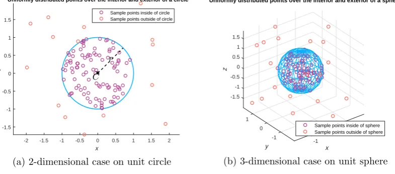
Unlike the original ABC algorithm, we use adaptive swarm size in this study. Gener-ally, the metaheuristics that use the adaptive swarm size paradigm generate a uniformly distributed population over the whole search space. However, if a solution is abandoned in ABC algorithm, then the generating a new bee population around the abandoned solu-tion is an unnecessary process leading waste of time. To prevent the mensolu-tioned case, we propose the generating a new population uniformly distributed on the interior or exterior of a hypersphere as a subdomain of whole search space. The incomplete gamma function allows us to perform the randomization process using Eq. 6.
~
pi=C~ +r. ~Ui S2
i
R
0
t(D2−1)e−tdt
!D1
Si.Γ D2
D1
whereU~i is randomly generated vector by continuous uniform distribution over the search space. C~ represents the position of best solution so far as the center of hypersphere, and
r is the radius of the hypersphere. In Eq. 6, Si =
v u u t
D
X
j=1
p2i,j for i= 1,2, . . . M such that M denotes the size of new population, and D specifies the dimension of search space. Eventually,~pi is the position ofith individual belonging the new generated population as a neural network parameter. Figure 1 illustrates the randomization process on a hyper-sphere. In Figure 1a, the generation of uniformly distributed points on the unit circle are demonstrated. Figure 1b repeats the demonstration on a unit sphere.
-2 -1.5 -1 -0.5 0 0.5 1 1.5 2 x
-1.5 -1 -0.5 0 0.5 1 1.5
y
Uniformly distributed points over the interior and exterior of a circle
Sample points inside of circle Sample points outside of circle
(a) 2-dimensional case on unit circle
-1.5 -1 -0.5
1 0
z
0.5
1
Uniformly distributed points over the interior and exterior of a sphere
y
0 1
x
1.5
0 -1
-1
Sample points inside of sphere Sample points outside of sphere
(b) 3-dimensional case on unit sphere
Figure 1. Uniformly distributed points generated randomly on the inte-rior or exteinte-rior of an hypersphere.
In our study, we generate a new bee population around the best solution ever found using Eq. 6 in each iteration. It applies exploitation by making a pressure to obtain better solution rather than the best found so far. Moreover, we generate a new candidate solution on the exterior of the neighbourhood of any abandoned solution, in the scout bee phase. After new population is generated the elitism stage is applied. In elitism, the fitness values of newly generated population is calculated, and the weakest ones are eliminated. The process maximises the probability of exploring the global optimum over the whole of search space. In each iteration, we also reduce the radius of the hypersphere by a damping ratio for making dynamization of exploration. The modified algorithm of ABC for obtaining the solution of the first order differential equations with initial conditions is given following in Algorithm 2 using the common functions given in Algorithm 1. One can easily update the cost function and the other related functions in Algorithm 2 for second order ODEs. In the next section, some different types of ODEs are solved numerically.
4. Numerical Experiments
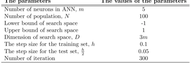
In the numerical experiments, we solve some types of initial value problems with FNN by training with both of classical and our proposed ABC algorithm. In all experiment, all the parameters used in FNN trained by ABC algorithm are selected identical as seen in Table 1 for making robust comparison.
Algorithm 1 Common functions used in ABC for IVPs
1: functionNet(t,~α,w~,β~) .returns the neural net solution att
2: m←the length of~α .mindicates the number of neurons in the NN.
3: return Pm
i=1αiσ(wit+βi) 4: end function
5: functiondNet(t,~α,w~,β~) .returns the derivation of neural net solution att
6: m←the length of~α .mindicates the number of neurons in the NN.
7: return Pm
i=1αiwiσ(wit+βi)(1−σ(wit+βi)) 8: end function
9: functionTrialy(t,t0,y0,p~) . returns the trial solution att according to the parameters of
neural network~p
10: return y0+ (t−t0)Net(t,~p) 11: end function
12: functiondTrialy(t,t0,y0,~p) .returns the value of ∂y∂tT
13: return Net(t,~α,w~,β~) +(t−t0)dNet(t,α~,w~,β~) 14: end function
15: functionCost(~t,t0,y0,~p) .returns the fitness value depending on all inputs
16: n←the length of vector~tspecifies the number of inputs
17: E← 1
n
n
X
j=1
{ dTrialy(tj,t0,y0,~p)−f(tj,Trialy(tj,t0,y0,~p))}2
18: return E
19: end function
Table 1. Free parameters used in this study.
The parameters The values of the parameters
Number of neurons in ANN,m 5
Number of population,N 100
Lower bound of search space -1
Upper bound of search space 1
Dimension of search space,D 3m
The step size for the training set,h 0.1
The step size for the test set, h2 0.05
Number of iteration 300
are used for training set. However, only the node given by initial conditions is belonging to the test set. After applying the training process to the network, it is able to give the numerical solution of any points in the interval.
Algorithm 2 Modified ABC Algorithm for IVP
1: procedureModified ABC IVP .Main code blocks of modified ABC for solving IVP
2: Specify the interval [a, b] as a search space
3: h←the step size .h >0
4: t0←a, y0←the initial condition for the problem
5: m←the number of neurons in Neural Net
6: Initialize the radius of hypersphere, r← |b−a|2
7: forj←0 tondo
8: tj ←a+hj .Create a partition of search space
9: end for
10: fori←1tomdo
11: Initialize artificial bee population as Neural Net parametersp~i = (~αi, ~βi, ~wi) such that
~
α, ~β, ~w∈Rm
12: Evaluate the fitness values for candidate solutions by calling Cost(~t,t0,y0,~pi) function
13: end for
14: iteration←1
15: repeat
16: for allemployeed beep~i do .employeed bee phase
17: Generate a new solution asp~0i in the neighbour of employeed bee~pi using the Eq. 3
wherekis randomly selected not equal toi
18: Evaluate the fitness values of new solutions by calling Cost(~t,x0,y0,p~0i) function
19: Apply the greedy selection by comparing the fitness values of new solutionsp~0
i and
fitness values of employeed bees~pi and determine the new population
20: end for
21: Check the probability values given Eq. 2 and normalize them to select onlooker bees
22: for allonlooker bee p~i do . onlooker bee phase
23: Generate new solution as p~0i in the neighbour of onlooker bee p~i according to the
probability valuePi
24: Evaluate the fitness values of new solutions by calling Cost(~t,x0,y0,p~0i) function
25: Apply the greedy selection by comparing the fitness values of new solutionsp~0i and
fitness values of onlooker beesp~i and determine the new population
26: end for
27: for allcandidate solutionp~i do .Scout bee phase
28: if the candidate is an abandoned solutionthen
29: Replace it with a new randomly produced solution satisfying the condition
PD
i=1(pi −Ci)2 > r2 for ensuring to stay the outside of the hypersphere as a neighboured
of the abandoned solution.
30: end if 31: end for
.Elitism phase
32: Using Eq. 6, generate a new bee population guaranteeing to stay inside of the
hyper-sphere as a neighboured of the best solution ever found.
33: Evaluate the fitness values of new solutions
34: Eliminate the weakest solutions according to the fitness values
35: Determine the best food source position and keep it into a memory.
36: Decrease the hypersphere radius by damping ratio
37: iteration←iteration +1
38: untilThe maximum number of iteration is reached
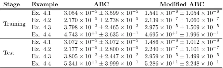
Furthermore, the best cost values encountered in each iteration of neural network train-ing stage are confronted. Figure 2 depicts the best cost values for each example. We also compare the execution time required for getting ODE solution in test stage. Algorithms are executed 10 times with randomly generated bee population, so the elapsed times are calculated for each execution. As a result, the mean and the standard deviation of the execution time is given in Table 7.
Example 4.1.
y0(t) + y(t)
t+ 1 = 0, t∈[2,4], y(2) = 3
(7)
The first example is first order homogenous linear differential equation as given in Eq. 7
having the exact solution asy(t) = 9
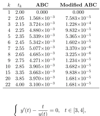
t+ 1. After 10 trials, the best cost values are calculated as1.568×10−5 and 4.240×10⁻⁹ for ABC and the modified version, respectively. Table 2 summarizes the obtained absolute errors for the problem.
Table 2. The absolute errors obtained from feed forward neural network outputs with test set using the step sizeh= 0.05 for Eq. 7 in Example 4.1.
k tk ABC Modified ABC
1 2.00 0.000 0.000
2 2.05 1.568×10⁻³ 7.583×10⁻⁵
3 2.15 3.724×10⁻³ 1.228×10⁻⁴
4 2.25 4.880×10⁻³ 9.832×10⁻⁵
5 2.35 5.339×10⁻³ 5.365×10⁻⁵
6 2.45 5.342×10⁻³ 1.602×10⁻⁵
7 2.55 5.077×10⁻³ 3.370×10⁻⁶
8 2.65 4.685×10⁻³ 3.225×10⁻⁶
9 2.75 4.271×10⁻³ 1.234×10⁻⁵
10 2.85 3.905×10⁻³ 3.682×10⁻⁵
15 3.35 3.663×10⁻³ 9.838×10⁻⁵
20 3.85 3.970×10⁻³ 1.681×10⁻⁵
22 4.00 3.100×10⁻³ 1.681×10⁻⁵
Example 4.2.
y0(t)− t
y(t) = 0, t∈[3,4], y(3) = 4
(8)
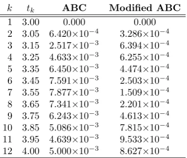
The First order homogenous linear differential equation as given in Eq. 8 has the exact solution as y(x) = √25−t2. The experiments show that the best cost values are 2.957× 10⁻⁵and3.099×10−7 for ABC and modified ABC orderly. The absolute errors are reported with Table 3, briefly.
Example 4.3.
y0(t) =−0.5(y(t)−25), x∈[0,15],
y(0) = 32 (9)
Table 3. The numerical solution of Feedforward Neural Network trained by ABC for test set in Example 2.
k tk ABC Modified ABC
1 3.00 0.000 0.000
2 3.05 6.420×10⁻⁴ 3.286×10⁻⁴
3 3.15 2.517×10⁻³ 6.394×10⁻⁴
4 3.25 4.633×10⁻³ 6.255×10⁻⁴
5 3.35 6.450×10⁻³ 4.474×10⁻⁴
6 3.45 7.591×10⁻³ 2.503×10⁻⁴
7 3.55 7.877×10⁻³ 1.509×10⁻⁴
8 3.65 7.341×10⁻³ 2.201×10⁻⁴
9 3.75 6.243×10⁻³ 4.613×10⁻⁴
10 3.85 5.086×10⁻³ 7.815×10⁻⁴
11 3.95 4.639×10⁻³ 9.533×10⁻⁴
12 4.00 5.000×10⁻³ 8.627×10⁻⁴
computed as 3.847×10⁻². This value is 2.173×10⁻⁵ for the modified version. Table 4 exposes the numerical errors by the mentioned methods.
Table 4. The numerical solution of Feedforward Neural Network trained by ABC for test set in Example 3.
k tk ABC Modified ABC
1 0.00 0.000 0.000
5 0.35 9.686×10⁻² 7.647×10⁻³
10 0.85 1.188×10⁻¹ 5.945×10⁻⁴
15 1.35 1.095×10⁻¹ 3.171×10⁻³
20 1.85 1.279×10⁻¹ 3.112×10⁻⁴
25 2.35 1.650×10⁻¹ 4.388×10⁻³
30 2.85 1.870×10⁻¹ 6.977×10⁻³
35 3.35 1.760×10⁻¹ 6.356×10⁻³
40 3.85 1.366×10⁻¹ 3.406×10⁻³
45 4.35 3.059×10⁻² 3.185×10⁻⁴
50 4.85 1.147×10⁻² 3.457×10⁻³
75 7.35 9.834×10⁻³ 1.155×10⁻³
100 9.85 2.192×10⁻¹ 6.211×10⁻³
125 12.35 3.464×10⁻¹ 5.451×10⁻³
150 14.85 1.883×10⁻¹ 4.640×10⁻³
152 15.00 1.692×10⁻¹ 6.936×10⁻³
Example 4.4.
y00(t)−5y0(t) + 4y(t) = 0, x∈[0,1], y(0) = 0
y0(0) =−1
(10)
In Eq. 10, second order homogenous linear differential equation with Cauchy condition
has the exact solution asy(t) = (exp(t)−exp(−4t))
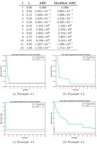
Table 5. The numerical solution of Feedforward Neural Network trained by ABC for test set in Example 4.
k tk ABC Modified ABC
1 0.00 0.000 0.000
2 0.05 2.951×10⁻² 2.965×10⁻²
3 0.15 1.893×10⁻¹ 1.908×10⁻¹
4 0.25 4.348×10⁻¹ 4.443×10⁻¹
5 0.35 8.301×10⁻¹ 8.397×10⁻¹
6 0.45 1.445×100 1.448×100
7 0.55 2.383×100 2.376×100
8 0.65 3.805×100 3.783×100
9 0.75 5.956×100 5.907×100
10 0.85 9.198×100 9.104×100
11 0.95 1.407×10+1 1.390×10+1
12 1.00 1.735×10+1 1.714×10+1
0 10 20 30 40 50 60 70 80 90 100 Iteration
0.047 0.048 0.049 0.05 0.051 0.052 0.053
Best cost so far
Cost values obtained from neural net solution
Modified ABC ABC
(a) Example 4.1
0 10 20 30 40 50 60 70 80 90 100 Iteration
0.051 0.052 0.053 0.054 0.055 0.056 0.057
Best cost so far
Cost values obtained from neural net solution
Modified ABC ABC
(b) Example 4.2
0 10 20 30 40 50 60 70 80 90 100 Iteration
0 0.1 0.2 0.3 0.4 0.5 0.6 0.7 0.8
Best cost so far
Cost values obtained from neural net solution
Modified ABC ABC
(c) Example 4.3
0 10 20 30 40 50 60 70 80 90 100 Iteration
2 3 4 5 6 7 8
Best cost so far
Cost values obtained from neural net solution
Modified ABC ABC
(d) Example 4.4
Figure 2. Graphs of best cost values found so far.
5. Conclusion
Table 6. Mean of cost values encountered in both training and testing stages.
Stage Example ABC Modified ABC
Training
Ex. 4.1 3.054×10⁻⁵±3.599×10⁻⁵ 1.541×10⁻⁸±1.054×10⁻⁸
Ex. 4.2 2.170×10⁻⁵±2.738×10⁻⁵ 2.139×10⁻⁷±1.060×10⁻⁷
Ex. 4.3 3.798×10⁻²±2.465×10⁻² 2.975×10⁻⁵±1.509×10⁻⁵
Ex. 4.4 4.743×10+1±3.635×10⁻¹ 4.695×10+1±1.996×10⁻¹
Test
Ex. 4.1 3.072×10⁻⁵±3.072×10⁻⁵ 1.486×10⁻⁸±1.012×10⁻⁸
Ex. 4.2 2.177×10⁻⁵±2.800×10⁻⁵ 2.240×10⁻⁷±1.101×10⁻⁷
Ex. 4.3 3.805×10⁻²±2.447×10⁻² 2.959×10⁻⁵±1.499×10⁻⁵
Ex. 4.4 5.341×10+1±3.999×10⁻¹ 5.286×10+1±2.248×10⁻¹
Table 7. Mean of elapsed time in seconds for test set.
Example ABC Modified ABC
Ex. 4.1 1.510×10⁻⁴±1.162×10⁻⁴ 1.516×10⁻⁴±1.344×10⁻⁴
Ex. 4.2 2.134×10⁻⁴±2.883×10⁻⁴ 1.775×10⁻⁴±2.105×10⁻⁴
Ex. 4.3 3.853×10⁻⁴±1.562×10⁻⁴ 4.681×10⁻⁴±2.267×10⁻⁴
Ex. 4.4 1.745×10⁻⁴±2.120×10⁻⁴ 1.429×10⁻⁴±1.289×10⁻⁴
function, we trained the network both traditional Artificial Bee Colony algorithm and a variant of ABC proposed by us. Proposed algorithm uses dynamically constructed hy-persphere to generate new bee population. The individuals in new population fall into the hypersphere to increase the exploitation ability of traditional ABC. Similarly, the individuals generated outside of the hypersphere supports the exploration quality of ABC. In this work, we give some numerical examples some different types of differential equa-tions such as first order and second order ODEs. The empirical studies precisely clarify that the modified version of ABC outperforms the classical ABC by means of absolute and mean squared errors. Table 6 exposes that cost values obtained in training and the testing stages are quite similar. Only, the desired improvement has not been achieved for the second order differential equation. Furthermore, it can be observed that the improvement has been drastic at the initial steps of the algorithm with Figure 2. However, it has been slight for following steps of the proposed algorithm.
According to the Table 7, the modification over classification does not affect the running time of the algorithm. The solution at each node of the interval [a, b] are reached as short as 10-thousandth of a second approximately. Consequently, the proposed metaheuristic provides an advancement to ABC algorithm. In addition, the mentioned suggestions can be applied to other population based global optimization algorithms as a future work.
Acknowledgement
We would like to acknowledge the support for this project from the Council of Higher Education in Turkey (Y ¨OK), Coordination of Academic Member Training Program ( ¨OYP) in Adnan Menderes University, under Grant no. AD ¨U- ¨OYP-14011.
References
[1] Lee, H. and Kang, I. 1990. Neural algorithms for solving differential equations, Journal of Computa-tional Physics, 91, 110.
[3] Lagaris, I. E., Likas, A. and Fotiadis, D. I. 1998. Artificial neural networks for solving ordinary and partial differential equations, IEEE Transactions on Neural Networks, 9(5), 987-1000.
[4] Aarts, L. P. and Van Der Veer, P. 2008. Neural Network Method for Solving Partial Differential Equations, Neural Process. Lett., 14(3), 261-271.
[5] McFall, K. S. and Mahan, J. R. 2009. Artificial Neural Network Method for Solution of Boundary Value Problems With Exact Satisfaction of Arbitrary Boundary Conditions, IEEE Transactions On Neural Networks, 20(8).
[6] Beidokhti, R. S. and Malek A. 2009. Solving initial-boundary value problems for systems of PDE using NN and optimization techniques, Journal of the Franklin Institute, 346, 898–913.
[7] Tsoulos, G. I., Gavrillis, D. and Glavas, E. 2009. Solving differential equations with constructed neural networks, Neurocomputing, 72, 2385-2391.
[8] Anastassi, A. A. 2014. Constructing Runge–Kutta methods with the use of artificial neural networks, Neural Computing and Applications, 25, 229-236.
[9] Raja, M. A. Z., Manzar, M. A. and Raza, S. 2015. An efficient computational intelligence approach for solving fractional order Riccati equations using ANN and SQP, Applied Mathematical Modelling, 39, 3075-3093.
[10] Kumar, M. and Yadav, N. 2015. Numerical Solution of Bratu’s Problem Using Multilayer, Natl. Acad. Sci. Letter, 38(5), 425–428.
[11] Raja, M. A. Z., Khan J. A. and Chaudhary, N. I. 2016. Reliable numerical treatment of nonlinear singular Flierl–Petviashivili eq. for unbounded domain using ANN, GAs, and SQP, Applied Soft Computing, 38, 617-636.
[12] Karaboga, D. 2005. An Idea Based On Honey Bee Swarm for Numerical Optimization, Technical Report-TR06, Erciyes University, Engineering Faculty, Computer Engineering Department.
[13] Karaboga, D. and Akay, B. 2009. A comparative study of Artificial Bee Colony algorithm, Applied Mathematics and Computation, 214(1), 108-132.
[14] Chun-Feng, W., Kui, L. and Pei-Ping, S. 2014. Hybrid artificial bee colony algorithm and particle swarm search for global optimization, Hindawi Publishing Corporation, Mathematical Problems in Engineering, Article ID 832949, 8 pages.
Korhan G¨unelgraduated from Ege University as a mathematician. He received his one of the M.Sc. degrees in computer engineering from Dokuz Eylul University, and received the other one in applied mathematics from Adnan Menderes University. He completed his Ph.D. degree in computer science at the Department of Mathematics in Ege University. His interests revolve around natural language processing, artificial intelligence applied to education, global optimization and machine learning for solving differential equations. Currently he works as Assistant Professor at the Department of Mathematics in Adnan Menderes University.