Advances in Science and Technology Research Journal
Volume 10, No. 29, March 2016, pages 97–108
DOI: 10.12913/22998624/61937 Research Article
Received: 2015.12.15 Accepted: 2016.02.01 Published: 2016.03.01
SOLVING THE PROBLEM OF VEHICLE ROUTING BY EVOLUTIONARY
ALGORITHM
Remigiusz Romuald Iwańkowicz1, Zbigniew Sekulski1
1 Faculty of Maritime Technology and Transport, West Pomeranian University of Technology, Al. Piastów 41, 70-065 Szczecin, Poland, e-mail: [email protected], [email protected]
ABSTRACT
In the presented work the vehicle routing problem is formulated, which concerns planning the collection of wastes by one garbage truck from a certain number of col-lection points. The garbage truck begins its route in the base point, collects the load in subsequent collection points, then drives the wastes to the disposal site (landfill or sorting plant) and returns to the another visited collection points. The filled garbage truck each time goes to the disposal site. It returns to the base after driving wastes from all collection points. Optimization model is based on genetic algorithm where individual is the whole garbage collection plan. Permutation is proposed as the code of the individual.
Keywords: vehicle routing, travelling salesman, genetic algorithm.
INTRODUCTION
Many companies in manufacturing, trading and providing various services faces the problem of the proper organisation of the distribution of their products or access their customers’ network . The most often undertaken issue of this type in literature is the problem of one salesman, also known as the travelling salesman problem (TSP). The essence of
this issue can be exemplified by the work of a com -mercial agent as follows. The sales representative
of a company goes out of his office to visit a set
number of customers. He must visit all his custom-ers and do this precisely once, and then return to
the office. The order of visits to individual custom -ers is optional, however, the goal of the sales rep-resentative is to select the shortest road. If the road of the travelling salesman is presented in a form of a graph, the solution of the salesman’s task is the Hamilton cycle, that is the cycle in the graph, in which each vertex of the graph is visited only once
(apart from the first vertex, which is the beginning
and the end of the journey) (Figure 1). Finding the Hamilton cycle with the minimal sum of the edge weights is equivalent to the solution of TSP.
TSP is of a combinational nature and belongs to the NP-complete problems [16], what means
that despite a very simple definition, in case of a
large number of vertices, it is practically insolu-ble in a reasonainsolu-ble period of time. If we assume that the distance between the customer A and cus-tomer B is different than the one between the cus-tomer B and customer A, the sales representative visiting only 10 customers can choose one of over 3.6 million routes. For the set number N of the visited customers, the number of routes possible to perform is (N-1)!.
the determined city, thus for all salesmen (Figure
1). In addition, it is assumed that no salesman can visit cities served by other travellers.
In the operational researches, the problem
of one salesman can thus be treated as a specific
case of the problem of many salesmen, also called
the vehicle routing problem (VRP), which defi -nition establishes that m vehicles initially placed
in the depot has to deliver in the specified area
separate amounts of goods to n customers. Deter-mining the optimal route for the group of vehicles with the service of the group of users is the VRP problem. Fisher [10] describes VRP as the task
of finding “the efficient use of a fleet of vehicles
that must make a number of stops to pick up and/or deliver passengers or products”. The aim for solving such a task is to minimise the total transport costs. The solution of the classical VRP problem is a set of routes, which begin and end in the depot, and this meets the limitation that all customers are serviced only once. Transportation costs can be improved by reducing the total dis-tance travelled by vehicles and reduction of the required number of vehicles. Since VRP belongs to the NP-difficult problems, it is usually solved
using heuristic methods, which do not provide the
best solutions, but enable finding satisfactory so -lutions in the accepted period of time. Accurate algorithms can be effective only in case of prob-lems with a relatively small number of customers and vehicles.
The VRP class of tasks can be defined in
terms of optimisation involving the appointment of the solution of the m-salesmen problem tak-ing into account additional conditions dependtak-ing
on the specific task. The first ones to formulate
the issue from this class under the name of truck dispatching problem were Dantzig and Ramser
[7] modelling it in a form of the fleet of identi -cal trucks used to supply several gas stations with
liquid fuels with the minimal travelling distance in terms of the central base. They formulated the mathematical approach to the problem and pub-lished the algorithm of this solution. Another pio-neering work is the article published by Balinski and Quandt [4], in which the authors generalised the VRP task to the form of linear optimisation, which is commonly encountered in the area of transport means management: i.e., how to serve a set of customers geographically scattered around
the centrally located based using the fleet of
trucks of different capacities.
VRPs are all around us, in the sense that many consumer products, such as soft drinks, beer, bread, gourmet food, fuel and medicines are
de-livered to retail outlets by a fleet of trucks, whose
work is organised according to the prescribed plan of the vehicle movement. Public services can also use these systems in order to improve their logistic chain. The export of waste or cleaning the town take up an increasingly bigger part of the budget of local authorities. VRPs are also related to the effective use of resources of the company rendering transport services, and thus they are an important factor in reducing the costs of its opera-tion and increasing the economic effectiveness of business operations. Such a wide use in practice makes VRPs be recognised as one of the most
important problems in the field of transport, dis -tribution and logistics. For example, Laporte [14]
presents a classic definition of VRP, “the problem
of designing optimal delivery or collection routes from one or several depots to a number of geo-graphically scattered cities or customers, subject to side constraints” and discusses some approxi-mated algorithms for solution of these tasks.
The above presented basic task of VRP is the starting point for formulating other problems,
which are the modification of the basic task. This
is why the majority of real tasks of planning
ve-Fig. 1. Graphic illustration of feasible solutions for tasks (from the left): travelling salesman problem (TSP), vehicle routing problem (VRP), open vehicle routing problem (OVRP); circles mean bases, squares mean
Advances in Science and Technology Research Journal Vol. 10 (29), 2016
hicle routes is much more often complicated compared to the classic VRP. Among many dif-ferent varieties of the problem of laying vehicle routes, we can list, for example: the task of ar-ranging vehicle routes with the capacitated ve-hicle routing problem, a problem with time win-dows (VRPTW), vehicle routing problem with simultaneous pickup and delivery (VRRSPD), vehicle routing problem with stochastic demands (VRPSD), split delivery vehicle routing problem (SDVRP), vehicle routing problem with multiple trips (VRPMT), open vehicle routing problem (OVRP) or dynamic vehicle routing problem, on-line, (DVRP). In the next part we will discuss two of them more detailed: capacitated vehicle rout-ing problem CVRP and the open task OVRP.
In case of the task with the limited capac-ity of vehicles it is assumed that each of the m vehicles has a limited capacity (most often the same). When travelling, vehicles take loads in the next points, however, it is unacceptable to take a greater amount than it results from the adopted capacity constraints. In case of CVRP the task of the company is thus to provide all customers with the desired amount of goods in such a way as to meet all of the following conditions (Figure 1): • each customer can be visited only by one
ve-hicle, which will provide the whole desired amount of goods;
• the capacity of each used vehicle cannot be exceeded;
• the sum of costs (or lengths) of routes covered by all vehicles used for this purpose must be as small as possible.
In such formulated CVRP issue there may be a few optimisation problems, e.g.:
• division of all recipients of goods into subsets
(set partitioning models), from which each one will be assigned to one vehicle, which is owned by the company;
• determining the order of deliveries within the subset, assigned to each vehicle used by the
company, that is determining the vehicle flow (vehicle flow models).
From the statement published by De Jaege-re et al. [8] it Jaege-results that the tasks of the CVRP type in recent years were the most often studied problems in the area of VRP problems. It is rarely assumed that vehicles are incapacitated, except in cases where it is considered that one vehicle
has insignificant sizes, e.g. [9]. The latest studies
were published in: [2, 3, 6, 12, 18, 19, 20, 26, 21].
The recently published works indicating the new variant of CVRP; instead of minimising the whole distance (or travel time) treated as the goal, the sum of times of arrivals at the customers is minimized, e.g. [13, 22, 23]. According to [8] this subject, cumulative capacitated vehicle routing problem (CCVRP), was devoted with 2% of pub-lications.
In the open VRP (OVRP) it is not required for the vehicles to return to the main base/stor-age after the visit to the last customer (Figure 1). If they do not return, they have to visit the same customers in the reverse order. In addition, OVRP often has two optimisation goals: minimisation of the used vehicles and (with this optimum number of vehicles) the minimisation of the total distance (or time) of travel. In practice, an additional
prob-lem appears when the fleet of vehicles is not the
property of the mere company rendering services
or when the available fleet of vehicles is not able
to satisfy the demand of its customers, so that (a part) of the activity related to distribution is ordered to the supplier of logistics of third par-ties (third party logistics, 3PL) [24]. The OVRP solution indicates then the number of vehicles, which are needed to perform the service/order. Moreover, OVRP can be used in case of the pick-up and delivery, when after delivery of goods to the given customers, vehicles receive the goods from the same customers, but in the reverse or-der [25]. In real life, OVRP occurs, for example, in the case of delivery to home of packages and magazines [24], school bus [25], route of output in coal mines [27] or transport of hazardous ma-terials [17].
According to the statement published by De Jaegere et al. [8] 6,25% of all publications on VRP contain OVRP as the main subject. Gener-ally speaking, all articles contain limitations of capacity for vehicles; in addition, more than half of articles includes limitations of the distance or time. All works, except for one [15], assume
a uniform fleet of vehicles and all except for [5]
adopt deterministic requirements. All proposed methods of the solution are meta-heuristics,
ex-cept for one [15] assume a uniform fleet of ve -hicles, and all except for one [27] were tested on the benchmark, the one adopted from literature or developed by authors.
Besides the fact that problems of the VRP type are among the most important problems of operational researches, in practice VRPs are also
They are very close to one of the most known combinational optimisation problems, the travel-ling salesperson problem (TSP), where only one person must visit all customers. Because TSP is a NP-difficult task, some researches formulate an opinion that we will never find the computa -tional technique, which will ensure the optimal solutions of such tasks, especially in case of large dimensions of the formulated tasks. VRP is even
more complicated. Even for small fleets and the
moderate number of visited points, the planning task is very complex. Therefore, it is not surpris-ing that people involved in plannsurpris-ing often turn to simple, local rules of vehicle routing.
Attempts to formulate the VRP tasks possibly close to real conditions usually lead to nonlinear tasks of combinatorial optimisation with many limitations, and most of the solution methods pro-posed so far cannot be effectively used for real tasks. Generally, meta-heuristics ensure much better solutions in real cases of large scale tasks. Gendreau et al. [11] discuss the use of meta-heu-ristics for VRP.
A characteristic feature of vehicle routing
problems is the ease of formulation of a specific
problem, as opposed to its solution. Hence, these issues interest many researchers, what results in
a significant number of proposed algorithms for
searching the best solutions. An interesting alter-native for the most popular methods of solving tasks of vehicle routing are evolutionary algo-rithms. These are methods intended primarily for solving the optimisation tasks, however, they ap-pear to be particularly useful in case of issues of the combinatorial nature. VRP solutions usually assessed by means of such dimensions as: the to-tal cost, distance, time of travel, number of used vehicles. Such a task should be treated as a multi-criteria optimisation task. In the paper we will
confine ourselves to solving a one-criterion task
of minimising the distance. The multi-criteria op-timisation task will be solved in the next publica-tions. The authors also plan to undertake studies to search for an optimal solution of the task using many vehicles.
VRP is the NP−difficult task of the combina -torial optimisation, which can be solved exactly only in the case of small-sized task. Although the heuristic approach does not guarantee optimal-ity, it gives satisfactory results in practice. In the last twenty years, meta-heuristics appeared as the most promising direction of studies for the family of VRP tasks.
PROBLEM FORMULATION
It is assumed that the research subject will involve the company, which provides services related to the collection and management of mu-nicipal waste, construction and industrial wastes, electrical and electronic equipment waste, recy-clables, bulky waste. The presented work formu-lated the problem of the collection of waste from containers located in a certain number of col-lection points located in different places of the adopted area by one specialised vehicle/garbage truck. It was assumed that in the adopted spatial area a perpendicular net was placed, whose sec-tions represent the potential secsec-tions of vehicle routes. In the selected grid nodes there are con-tainers, where the determined volume of waste is located. It was assumed that the garbage truck, with the adopted capacity of the trailer, collects the load while driving through next (according to the movement plan) collection points. After
filling the trailer in a degree preventing the ser -vice of the next point, the vehicle stops its waste collection and drives the waste through the shortest path to the disposal side or garbage util-isation location to dispose the trailer. The empty vehicle returns to the adopted area and begins the next working cycle visiting other collection points and collecting waste in them. After each
filling of the trailer, the full garbage truck drives
to the place of storage of disposal. The garbage truck returns to the base point after collecting and driving to the storage or disposal place waste collected in all reception points. Such a formulated task is a VRP task and in particular it has features of two VRP types: capacitated ve-hicle routing problem (CVRP) and open veve-hicle routing problem (OVRP). Doubts can be raised by the fact of classifying the formulated task to the VRP class, if only one vehicle participates in the movement, as it happens in case of the travelling salesman problem (TSP). However, it will be demonstrated that the solution of the for-mulated problem is the plan of the garbage truck operation with the nature of the cycle collection, which can be successfully serviced by several vehicles in parallel.
MATHEMATICAL MODEL
prob-Advances in Science and Technology Research Journal Vol. 10 (29), 2016
lem was initiated from adopting the following as-sumptions:
• unsorted household waste will be collected in the collection points,
• waste will be collected within one working day,
• for the collection of waste one specialised ve-hicle will be used, a garbage truck, with the
fixed capacity of the container V,
• the number of waste collection points N is
fixed,
• the volume of waste v1, v2, ..., vN, which should be collected from the collection points on the given day are random variables, and after the adoption these values are established and con-stitute the model parameters,
• each collection point can be served by the gar-bage truck with the assumed capacity of the trailer:
1,2,..., :
ii
N v V
∀ =
≤
(1)• during the whole process, the garbage truck visits each collection point only once, in order to collect the whole volume of waste accumu-lated at a given point,
• the base point and collection points are located on the plane, and their location is given by the Euclidean coordinates (the beginning of the Cartesian coordinate system is located at the base point with Euclidian coordinates (x0, y0), collection points in the points with coordinates (x1, y1), (x2, y2), ..., (xi, yi), ..., (xN, yN) and the disposal site in the point with coordinates (xN+1, yN+1); coordinates of points are determined in the task and constitute the parameters of the optimisation task,
• the need to refuel and the occurrence of other interference of the garbage truck operation during the whole process of waste collection are omitted,
• the occurrence of potential traffic problems is
omitted: congestion, repairs, breakdowns, de-tours.
It is assumed that the road infrastructure,
which will be used by the vehicle, is fixed and
known. So you can determine the distance be-tween points with the empirical or theoretical method. Mutual distances between the base point and the collection points, between the collection points and the disposal site, and the collection points are known and they can be written down in a form of the distance matrix. The general dis-tance matrix takes the form of:
operation with the nature of the cycle collection, which can be successfully serviced by several vehicles in parallel.
3 Mathematical model
Formulation of the mathematical model of the waste collection by the garbage truck problem was initiated from adopting the following assumptions:
unsorted household waste will be collected in the collection points,
waste will be collected within one working day,
for the collection of waste one specialised vehicle will be used, a garbage truck, with the
fixed capacity of the container V,
the number of waste collection points N is fixed,
the volume of waste v1, v2, ..., vN, which should be collected from the collection points on the given day are random variables, and after adoption these values are established and constitute the model parameters,
each collection point can be served by the garbage truck with the assumed capacity of the
trailer:
1,2,..., : i
i N v V
(1)
during the whole process, the garbage truck visits only once each collection point, in order
to collect the whole volume of waste accumulated at a given point,
the base point and collection points are located on the plane, and their location is given by
the Euclidean coordinates (the beginning of the Cartesian coordinate system is located at
the base point with Euclidian coordinates (x0, y0), collection points in the points with
coordinates (x1, y1), (x2, y2), ..., (xi, yi), ..., (xN, yN) and the disposal site in the point with coordinates (xN+1, yN+1); coordinates of points are determined in the task and constitute the
parameters of the optimisation task,
the need to refuel and the occurrence of other interference of the garbage truck operation
during the whole process of waste collection are omitted,
the occurrence of potential traffic problems is omitted: congestion, repairs, breakdowns,
detours.
It is assumed that the road infrastructure, which will be used by the vehicle, is fixed and known. So you can determine the distance between points with the empirical or theoretical method. Mutual distances between the base point and the collection points, between the collection points and the disposal site, and the collection points are known and they can be written down in the form of the distance matrix. The general distance matrix takes the form of:
0,1 0,2 0, 0, 1
1,0 1,2 1, 1, 1
2,0 2,1 2, 2, 1
,0 ,1 ,2 , 1
1,0 1,1 1,2 1.
base col. p. 1 col. p. 2 col. p. disp. site base
col. p. 1 col. p. 2
col. p. disp. site 0 0 0 0 0 N N N N N N
N N N N N
N N N N N
N
N
d d d d
d d d d
d d d d
d d d d
d d d d
D (2)
Distances determined empirically are of course more accurate, as they take into account the real course of routes. For the purposes of the undertaken studies we used distances determined course more accurate, as they take into account Distances determined empirically are of
the real course of routes. For the purposes of the undertaken studies we used distances determined theoretically based on Cartesian coordinates of the points. Depending on the adopted metrics, these distances can have various values. The commonly used distance measure in the Euclid-ean space is the Minkowski metrics in a form of:
{
}
,(
)
1, 0,1,2,..., , 1 : i j i j r i j r r
i j N N d x x y y
∀ ∈ + = − + −
{
}
,(
)
1, 0,1,2,..., , 1 : i j i j r i j r r
i j N N d x x y y
∀ ∈ + = − + − (3)
Adopting the Minkowski metrics, it is as-sumed that the distance between the points is symmetrical (di,j = dj,i). It is a general metric, where r constitutes the parameter. For r = 1 the Minkowski metrics takes the form of the taxicab distance, while for r = 2 the form of the Euclid-ean measure. In case of waste collection within the city, it is advisable to adopt the taxicab dis-tance (also called Manhattan). The disdis-tance of two points in this metrics is the sum of absolute values of differences of their coordinates:
{
}
,,
0,1,2,..., ,
1 :
Ti j i j i j
i j
N N
d
x x
y y
∀
∈
+
=
−
+
−
{
}
,,
0,1,2,..., ,
1 :
Ti j i j i j
i j
N N
d
x x
y y
∀
∈
+
=
−
+
−
(4)The characteristic feature of the taxicab dis-tance is the fact that for the determined pair of points (i, j) there may be many different paths with the length of di,j. These are the shortest roads (i.e. minimal) and it does not matter which will be chosen by the driver (Figure 2).
The formulated optimisation task should in-clude: decision variables, optimisation criterion, limitations, parameters.
Decision variables
points is determined as follows:
(
p1, ,.p2 ..,pN)
, i{
1,2,...,N}
: pi{
1,2,...,N}
= ∀ ∈ ∈
p
(
p1, ,.p2 ..,pN)
, i{
1,2,...,N}
: pi{
1,2,...,N}
= ∀ ∈ ∈
p (5)
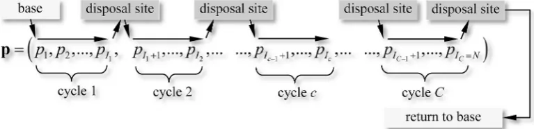
The interpretation of the decision variant rep-resented by vector p requires consideration of the garbage truck capacity V and the capacity of waste in the collection points: v1, v2, ..., vN. In gen-eral, the whole waste collection process is divided into three cycles (Fig. 3.):
• Cycle c = 1.: the garbage truck starts from the base point, visits I1 collection points with numbers p p1, ,...,2 pI1 (of course
1 2 ... I1
p p p
v +v + +v ≤V), and then goes
through the minimal route from the point numbered pI1 to the disposal site.
• Cycle c ∈ {2, 3, ..., C}: starting from the dispos-al site, the garbage truck visits the collection points numbered pIc−1+1,pIc−1+2,...,pIc−1,pIc
and after each filling of the trailer it goes to
the disposal site.
Numbers I1, I2, ..., IC are the border indices of elements of vector p. After receiving waste from the points numbered p pI1, I2,...,pIC the garbage truck travels to the disposal site.
In each cycle the garbage truck visits as many collection points, so the total capacity of waste does not exceed truck capacity. At the same time,
it seeks the maximal fill of the working space of the garbage truck. As a result, for the fixed cycle c and index Ic-1 in vector p of the last number of the point visited in the previous cycle (this is number
1 c I
p −) it is possible to determine the index Ic of the number pIc of the last visited point in the cycle c. This is the index satisfying the condition:
1 1
1
0
1 1
1,2,...,
1:
c i c i,
0
c c
I I
p p
i I i I
c
C
v
V
v
I
− −
+
= + = +
∀ =
−
∑
≤ <
∑
=
1 1
1
0
1 1
1,2,...,
1:
c i c i,
0
c c
I I
p p
i I i I
c
C
v
V
v
I
− −
+
= + = +
∀ =
−
∑
≤ <
∑
=
(6)Next indices Ic are determined recursively starting from c = 1. The number of cycles is deter-mined dynamically during calculations of subse-quent indices. The number of the last cycle is cal-culated when for some cycle numbered c waste
collected in all other collection points fit into the
garbage truck:
1
1,2,...:
i1
c N
p i I
c
v
V
C c
= +
=
∑
≤
⇒
= +
(7)The C cycle differs from the previous ones in that the waste amount collected by the garbage truck is the residue remaining in the collection
points and can fill only a small part of the cargo
space. The string of indices is written in a form of a vector: I = (I1, I2, ..., IC).
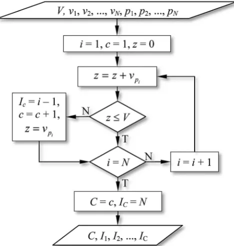
The algorithm performing the decoding oper-ation of the decision variables vector p on the real plan of collection and export of waste can adopt the form presented in Figure 4.
During next iterations i = 1, 2, ..., N the state of the garbage truck load z is controlled. If it ex-ceeds the volume V, then the cycle end index is determined, as well as the number of the next cycle and the new load state. Reaching the last iteration (i = N) allows to determine the number of all operation cycles of the garbage truck C.
Optimisation criterion
The optimisation criterion is the minimisa-tion of the whole route covered by the garbage truck during the process of waste collection from all points and their delivery to the disposal site.
Fig. 3. The idea of the waste collection process divided into cycles adopted in the paper
Advances in Science and Technology Research Journal Vol. 10 (29), 2016
The base point is the starting and ending point of the path. For the determined vector of permutation of collection points numbers p, using the decoding algorithm (Figure 4) and the given distance matrix
D (formula 2) it is possible to calculate the total length of the route travelled by the garbage truck:
( )
(
)
( )
1 1 2 2 3 11 1 11 1 2 2 3 1
1 1 1 1 1 2 2 2
1 1 2 2 3 1
2 2 2 2 2 3 3 3
1
1 1
0, , , , , 1
1, , , , , 1
1, , , , , 1
1,
, ...
... ... ...
I I I
I I I I I I I I
I I I I I I I I
IC IC
p p p p p p p p N
N p p p p p p p p N
N p p p p p p p p N
N p p
L L d d d d d
d d d d d
d d d d d
d d − + + + + + − + + + + + − + − − + + + + + + = = + + + + + + + + + + + + + + + + + + + + + +
p I p p
1, 12 12, 13 1, , 1
1,0
...
IC IC IC IC IC IC
p p p p p p N
N
d d d
d + ++ −+ −+ − + + + + + + + + ( )
(
)
( ) 1 1 2 2 3 11 1 11 1 2 2 3 1
1 1 1 1 1 2 2 2
1 1 2 2 3 1
2 2 2 2 2 3 3 3
1
1 1
0, , , , , 1
1, , , , , 1
1, , , , , 1
1,
, ...
... ... ...
I I I
I I I I I I I I
I I I I I I I I
IC IC
p p p p p p p p N
N p p p p p p p p N
N p p p p p p p p N
N p p
L L d d d d d
d d d d d
d d d d d
d d − + + + + + − + + + + + − + − − + + + + + + = = + + + + + + + + + + + + + + + + + + + + + +
p I p p
1, 12 12, 13 1, , 1
1,0
...
IC IC IC IC IC IC p p p p p p N
N
d d d
d
+ ++ −+ −+ − +
+
+ + + + +
+
The above sum was written in a way that
facilitates the identification of subsequent work
cycles (rows 1, 2, ..., C of the equation) and the
route back to the base (the last row). The first
component of the sum (8) is the distance from the
base to the first collection point. Further compo
-nents in the first column represent distances from the landfill to the first collection point in the cycle
or to the base (the last component). In the last col-umn there are distances from the last collection
point visited during the cycle to the landfill.
The optimisation criterion in the selection process of the permutation vector p is the mini-misation of the route length L(p). The adoption of this criterion enables writing the function of goal in a form of:
( )
1 1 11
1 1
0, , , 1 1, 1,0 0
1 1 1 1
min,
0
c
k k Ic Ic
c I
C C C
p p p p N N p N
c k I c c
L
d
d
+d
d
+d
I
− − − + + + = = + = =
=
+
∑ ∑
+
∑
+
∑
+
→
=
p
( )
1 1 11
1 1
0, , , 1 1, 1,0 0
1 1 1 1
min,
0
c
k k Ic Ic
c I
C C C
p p p p N N p N
c k I c c
L
d
d
+d
d
+d
I
−
− −
+ + +
= = + = =
=
+
∑ ∑
+
∑
+
∑
+
→
=
p
(9)The implementation of the above criterion en-sures integration of planning of individual work cycles. The unfavourable phenomenon of not
filling the garbage truck capacity in the cycles is
punished by the adopted criterion by the increased number of cycles and as a result the prolongation of the total route.
Constraints
The set of feasible solutions is the set of all permutations of the set of collection point num-bers {1, 2, ..., N}. Each permutation is allowed. As a result, the space of searching includes n! of decision variants. So, here we can see the effect of explosion of the search space with the increase of the number of collection points.
Parameters of the model
Parameters of the optimisation model are: number of vehicles m = 1, garbage truck capacity V = 18 m3, coordinates of the base point (x
0, y0), collection points (x1, y1), (x2, y2), ..., (xi, yi), ..., (xN, yN) and the disposal site (xN+1, yN+1), capacity of waste in collection points: v1, v2, ..., vN.
Fig. 4. The algorithm used in the paper generating the border indices of connection points numbers ending the garbage truck operation cycles
The standard capacity of the garbage truck is in the range between 18 and 22 m3. The waste container has the volume of 1.5 m3. In the single collection point there are most often two contain-ers. This means that in each collection point there are at most 3.0 m3 of waste.
OPTIMISATION METHOD
The problem is combinatorial in nature. For this reason, it is advisable to use the evolutionary algorithm, as the search method for the optimal solution. In this case this solution involves the permutation of collection points numbers arrang-ing them in the order of garbage truck visits.
The permutation coding of the travelling salesman problem is the standard approach [1]. The subject is represented by the string of N num-bers, which is a permutation of the set {1, 2, ..., N}. The proposed evolutionary algorithm con-tains the following genetic operators:
• generating the first population by drawing a
random even number G of random N-element permutations,
• assessment of the adaptation of individuals based on the objective function (9). The deter-mined even number E of the best adapted indi-viduals in the population is treated as an elite, • the selection of parents from the population
with the proportional method (roulette). There are GE pairs of parents drawn. Each pair of parents generates one child,
• crossing chromosomes of parents with the “or -der crossover” method. The chromosome of the child is generated according to the scheme: – drawing the crossing point,
– the part of the parent chromosome 1 to the left (or right) from the crossing point re-mains unchanged,
– the second part of the chromosome is sort-ed according to the order of occurrence in the parent chromosome 2.
• the mutation of child chromosome involves drawing the pair of genes (numbers of col-lection points) and changing their places in the permutation vector p. The mutation takes place with a certain probability,
• the recording of the next population as the sum of the set of elite individuals and the set of offspring subjected to the mutation operator.
After filling the set of offspring with elite indi -viduals, the new population has G individuals.
EXAMPLE STUDY
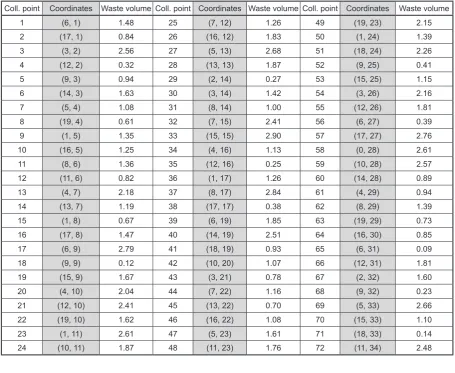
Using the previously formulated optimisation model of the VRP task, the calculation example was used assuming 72 collection points distrib-uted with the base point and the disposal site on the grid measuring 20 to 35 units. The randomly adopted coordinates of the collection points and the waste volume in these points are presented in Table 1.
The base point has coordinates (0, 0) and the disposal site (20, 35). Based on points coordinates it is possible to determine the distance matrix D. The Manhattan measure was adopted.
After conducting test calculations for differ-ent values of parameters controlling the algorithm it was assumed that the satisfactory convergence was achieved by the evolutionary algorithm for the following parameters:
• number of the populations: G = 40; • number of elite units: E = 6; • probability of mutation: 0.2; • roulette scaling exponent: 2.
In Figure 5 the history of adaptation function evolution is presented.
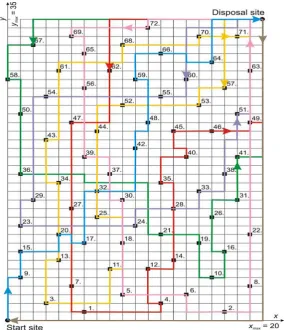
It can be seen that in the course of the simula-tion, the function achieved saturation. The whole time of simulation was used to improve the adap-tation function, what means the ongoing improve-ment of the best solutions searched by the algo-rithm. The lowest function value was obtained in the 4132 generation. The variant with such a function value was adopted as the searched opti-mal variant. The objective function value (route length) for the above solution is: L = 612 m. The best found solution is the following order of the visited collection points with the division into 6 cycles (B – base point, D – disposal site):
• Cycle 1: B, 9, 15, 20, 17, 32, 42, 48, 59, 66, 64, D;
• Cycle 2: D, 67, 58, 50, 36, 21, 19, 10, 16, 26, 31, 41, D;
• Cycle 3: D, 57, 53, 52, 44, 25, 18, 11, 3, 13, 34, 43, 61, 68, 70, 71, D;
• Cycle 4: D, 62, 47, 27, 7, 1, 4, 12, 14, 35, 40, 45, 46, 49, D;
• Cycle 5: D, 60, 55, 54, 29, 23, 24, 28, 33, 38, 51, 63, D;
• Cycle 6: D, 72, 69, 65, 56, 39, 37, 30, 5, 6, 2, 8, 22, D.
en-Advances in Science and Technology Research Journal Vol. 10 (29), 2016
vironment of the Matlab program. The PC class computer (3 GHz, 4 GB RAM) performed calcu-lations of one simulation for about 10 seconds.
The optimal route of the garbage truck was shown in Figure 6. Each cycle is marked with different colour. After ending the sixth cycle, the garbage truck returns to the base point.
The garbage truck loading condition in each cycle changes with the visit of next collection points. After ending the cycle, the garbage truck
unloads waste in the disposal site and its loading condition returns to the level 0. In Figure 7 the dynamics of the loading condition was presented for the optimal solution. As it can be seen, in each cycle the garbage truck gets the level of loading close to maximal V = 18 m3.
It can be noticed that the order of execution of the starting and ending cycles in the disposal site does not matter. In the considered example there are 5 such cycles, so the agreed optimal plan can Table 1. The list of adopted collection points, their coordinates and waste volume
Coll. point Coordinates Waste volume Coll. point Coordinates Waste volume Coll. point Coordinates Waste volume 1 (6, 1) 1.48 25 (7, 12) 1.26 49 (19, 23) 2.15 2 (17, 1) 0.84 26 (16, 12) 1.83 50 (1, 24) 1.39 3 (3, 2) 2.56 27 (5, 13) 2.68 51 (18, 24) 2.26 4 (12, 2) 0.32 28 (13, 13) 1.87 52 (9, 25) 0.41 5 (9, 3) 0.94 29 (2, 14) 0.27 53 (15, 25) 1.15 6 (14, 3) 1.63 30 (3, 14) 1.42 54 (3, 26) 2.16 7 (5, 4) 1.08 31 (8, 14) 1.00 55 (12, 26) 1.81 8 (19, 4) 0.61 32 (7, 15) 2.41 56 (6, 27) 0.39 9 (1, 5) 1.35 33 (15, 15) 2.90 57 (17, 27) 2.76 10 (16, 5) 1.25 34 (4, 16) 1.13 58 (0, 28) 2.61 11 (8, 6) 1.36 35 (12, 16) 0.25 59 (10, 28) 2.57 12 (11, 6) 0.82 36 (1, 17) 1.26 60 (14, 28) 0.89 13 (4, 7) 2.18 37 (8, 17) 2.84 61 (4, 29) 0.94 14 (13, 7) 1.19 38 (17, 17) 0.38 62 (8, 29) 1.39 15 (1, 8) 0.67 39 (6, 19) 1.85 63 (19, 29) 0.73 16 (17, 8) 1.47 40 (14, 19) 2.51 64 (16, 30) 0.85 17 (6, 9) 2.79 41 (18, 19) 0.93 65 (6, 31) 0.09 18 (9, 9) 0.12 42 (10, 20) 1.07 66 (12, 31) 1.81 19 (15, 9) 1.67 43 (3, 21) 0.78 67 (2, 32) 1.60 20 (4, 10) 2.04 44 (7, 22) 1.16 68 (9, 32) 0.23 21 (12, 10) 2.41 45 (13, 22) 0.70 69 (5, 33) 2.66 22 (19, 10) 1.62 46 (16, 22) 1.08 70 (15, 33) 1.10 23 (1, 11) 2.61 47 (5, 23) 1.61 71 (18, 33) 0.14 24 (10, 11) 1.87 48 (11, 23) 1.76 72 (11, 34) 2.48
be implemented in 5! ways. All are considered in terms of the objective function value.
CONCLUSIONS
The article presented the concept of the plan-ning model for the order of waste collection by the garbage truck from the pre-set collection points. The model is based on the mechanism of searching the space of points numbers permuta-tion. The evolutionary algorithm was used for random searching of the focus. It was shown in the example that it is convergent with the optimal solution and that the criterion of the minimisation of the garbage truck route distance simultane-ously leads to the fullest loading of the vehicle in
Fig. 6. The optimal route of the garbage truck found in the paper, which collects waste in agreed collection points (collection points are marked with red squares in grid nodes and numbered: 1., 2., 3., etc.)
Fig. 7. The conditions of the garbage truck loading in next work cycles
each cycle. It is an advantageous phenomenon, it
simplifies the model and speeds up the optimisa -tion calcula-tions.
The proposed model is based on the assump-tion that we know the amounts of waste waiting in collection points. In practice, it is problematic to forecast these amounts. On the one hand, these are random variables and the forecast of their val-ue can be performed only with a certain probabil-ity. On the other hand, one should consider the fact that waste is crushed by the garbage truck, so their volume is changed. The degree of com-pressing waste is also a random variable, which depends on the type of waste.
Advances in Science and Technology Research Journal Vol. 10 (29), 2016
container content mass. Sensors can be placed, for example, in the elements of the drive chassis. However, it is an expensive solution. Such sen-sors would have to have the opportunity to send information remotely. The degree of waste com-pression is a variable, whose forecast can take place only based on historical data and the devel-oped statistical distributions.
An alternative approach for solving the above problems can be the use of the dynamic algorithm updating the garbage truck path after visiting each collection point and verifying the real condi-tion of the waste loading. Such an algorithm will be the subject of considerations and next publica-tions of authors.
The presented model is the result of prelimi-nary considerations of the authors. It does not include a number of complications occurring in practice, for example: the limited work time of the garbage truck staff, the need to refuel, the oc-currence of other interference of the garbage truck work during the whole waste collection process,
the potential traffic problems (e.g. congestion,
repairs, break-downs, detours). The one-criteria optimisation task was formed and solved, while the undertaken decision problem in reality is the multi-criteria problem (e.g. the minimisation of the number of used vehicles and the minimisation of the working time of one vehicle).
It is planned to establish contact with com-panies involved in waste management in order to identify conditions of the implementation of the optimisation model in practice. In addition to the analytical capabilities of the system, it will be necessary to take into account the issues of users’ interfaces, the way of data recording and com-munication between the disposition centre and vehicles.
REFERENCES
1. Abdoun O., Abouchabaka J. 2011. A comparative study of adaptive crossover operators for genetic algorithms to resolve the traveling salesman prob-lem. International Journal of Computer Applica-tions, 31(11), 49–57.
2. Ai T.J., Kachitvichyanukul V. 2009. A particle swarm optimization for the vehicle routing prob-lem with simultaneous pickup and delivery. Com-puters & Operations Research, 36(5), 1693–1702. 3. Baldacci R., Mingozzi A., Roberti R. 2012.
Re-cent exact algorithms for solving the vehicle rout-ing problem under capacity and time window
constraints. European Journal of Operational Re-search, 218(1), 1–6.
4. Balinski M., Quandt R. 1964. On an integer pro-gram for a delivery problem. Operations Research, 12, 300–304.
5. Cao E., Lai M. 2010. The open vehicle routing problem with fuzzy demands. Expert Systems with Applications, 37(3), 2405–2411.
6. Chen P., Huang H., Dong X.-Y. 2010. Iterated vari-able neighborhood descent algorithm for the ca-pacitated vehicle routing problem. Expert Systems with Applications, 37(2), 1620–1627.
7. Dantzig G.B., Ramser J.H. 1956. The truck dispatch-ing problem. Management Science, 6(1), 80–91. 8. De Jaegere N, Defraeye M, Van Nieuwenhuyse
I. 2014. The vehicle routing problem: state of
the art classification and review. Research Report
KBI_1415, Faculty of Economics and Business, Leuven, België.
9. Ferrucci F., Bock S., Gendreau M. 2013. A pro-active real-time control approach for dynamic ve-hicle routing problems dealing with the delivery of urgent goods. European Journal of Operational Research, 225(1), 130–141.
10. Fisher M. 1995. Vehicle routing. In: Handbooks of Operations Research and Management Science, Vol 8: Network Routing, Ball M.O., Magnanti T. L., Monoma C.L. and Nemhauser G.L. (Eds.), North-Holland, Amsterdam, 1–31.
11. Gendreau M., Potvin J.Y. Braysy O. Hasle G., Lok-ketangen A. 2008. Metaheuristics for the vehicle routing problem and its extensions: a categorized bibliography. In: B. Golden, S. Raghavan and E. Wasil (Eds.), The Vehicle Routing Problem – Lat-est Advances and New Challenges, Springer, Hei-delberg, 143–169.
12. Jin J., Crainic T.G., Løkketangen A. 2012. A paral-lel multi-neighborhood cooperative tabu search for capacitated vehicle routing problems. European Journal of Operational Research, 222(3), 441–451. 13. Ke L., Feng Z. 2013. A two-phase metaheuris-tic for the cumulative capacitated vehicle rout-ing problem. Computers & Operations Research, 40(2), 633–638.
14. Laporte G. 1992. The vehicle routing problem: An overview of exact and approximate algorithms. European Journal of Operational Research, 59(3), 345–358.
15. Li X., Leung S.C.H., Tian P. 2012. A multistart adap-tive memory-based tabu search algorithm for the
het-erogeneous fixed fleet open vehicle routing problem.
Expert Systems with Applications, 39(1), 365–374. 16. Lin S, Kernighan B.W. 1973. An effective heuristic
17. Liu R., Jiang Z. 2012. The close–open mixed ve-hicle routing problem. European Journal of Opera-tional Research, 220(2), 349–360.
18. Liu R., Jiang, Z., Fung R.Y.K., Chen F., Liu X. 2010. Two-phase heuristic algorithms for full truckloads multi-depot capacitated vehicle routing problem in carrier collaboration. Computers and Operations Research, 37(5), 950–959.
19. Lin S.-W., Lee Z.-J., Ying K.-C., and Lee C.-Y. 2009. Applying hybrid meta-heuristics for capaci-tated vehicle routing problem. Expert Systems with Applications, 36(2), 1505–1512.
20. Lysgaard J. 2010. The pyramidal capacitated ve-hicle routing problem. European Journal of Opera-tional Research, 205(1), 59–64.
21. Marinakis Y. (2012. Multiple Phase Neighborhood Search-GRASP for the Capacitated Vehicle Rout-ing Problem. Expert Systems with Applications, 39(8), 6807–6815.
22. Mattos Ribeiro G., Laporte G. 2012. An adaptive large neighborhood search heuristic for the cumu-lative capacitated vehicle routing problem.
Com-puters and Operations Research, 39(3), 728–735.
23. Ngueveu S. U., Prins C., Wolfler Calvo R. 2010.
An effective memetic algorithm for the cumulative capacitated vehicle routing problem. Computers & Operations Research, 37(11), 1877–1885.
24. Repoussis P.P., Tarantilis C.D. 2010. Solving the
fleet size and mix vehicle routing problem with
time windows via adaptive memory programming. Transportation Research Part C: Emerging Tech-nologies, 18(5), 695–712.
25. Salari M., Toth P., Tramontani A. 2010. An ILP im-provement procedure for the Open Vehicle Rout-ing Problem. Computers and Operations Research, 37(12), 2106–2120.
26. Szeto W.Y., Wu Y., Ho S.C. 2011. An artificial bee
colony algorithm for the capacitated vehicle rout-ing problem. European Journal of Operational Re-search, 215(1), 126–135.