APPLICATION OF THE MAXIMA IN THE TEACHING OF SCIENCE SUBJECTS AT DIFFERENT LEVELS OF KNOWLEDGE

(1)

44

Advances in Science and Technology Research Journal

Volume 8, No. 24, Dec. 2014, pages 44–50

DOI: 10.12913/22998624/566 Original Article

Received: 2014.10.18 Accepted: 2014.11.12 Published: 2014.12.01

APPLICATION OF THE MAXIMA IN THE TEACHING OF SCIENCE SUBJECTS

AT DIFFERENT LEVELS OF KNOWLEDGE

Anna Makarewicz1

1_{Department of Applied Mathematics, Lublin University of Technology, Nadbystrzycka 38, 20-618 Lublin,} Poland, e-mail: [email protected]

ABSTRACT

In this paper I present a program Maxima, which is one of the best computer algebra system (CAS). The program is easy to use and offers many possibilities. In the text the interface, basic commands, and various examples to facilitate complex calculations in

almost every field of mathematics are preented. I prove that the program can be used

in secondary schools, upper secondary schools and college. Program’s capabilities are presented, including, among others, differentiation and symbolic integration, symbol-ic solving equations (including differential), simplifying algebrasymbol-ic expressions, matrix operations, the possibility of drawing graphs of 2D / 3D and others.

Keywords: computer program, numerical computation, symbolic computation, sym-bolic differentiation, symsym-bolic integration, graph, graph three-dimensional, function.

INTRODUCTION

Maxima is a computer program, performing mathematical calculations, both symbolic and nu-meric. The use of symbolic computation allows to solve many mathematical problems in an accurate manner. Maxima can work as a calculator, which can be used in secondary schools. It is able to create very complex parametric function graphs, implicit function graphs and graphs of function of several variables, (with such problems faced students of almost all departments), these are nec-essary basics that form the base for further de-velopment and specialization in a specific area, for example mechanics, electrical engineering, computer science, construction, aviation, broadly understood technologies, etc.

This program stems from program macsyma developed at the Massachusetts Institute of Tech-nology for the Department of Energy. The soft-ware features include:

• performing numerical calculations with any accuracy,

• simplifying algebraic expressions and trigono-metric,

• symbolic solving equations (including differ-ential),

• symbolic solving systems of equations, • symbolic differentiation and integration, • matrix operations,

• drawing graphs of functions,

• perform calculations in the field of probability theory,

• define your own functions by the user,

• export of the results to the following formats: HTML, LaTeX, and graphic formats PNG, PostScript.

(2)

alter-45

Advances in Science and Technology Research Journal vol. 8 (23) 2014

native solutions and create visualization. It also helps to save time and to control and eliminate errors in solving complex accounting tasks.

BASICS MAXIMA

Maxima works at input %i and outputs %o. Inputs and outputs are numbered that in

combina-tion with the %i or %o creates a unique identifier.

Maxima distinguishes quantity of letter, so the function f(x) and F(x) are not the same. Variable %i stores the result of the last command.

Each instruction must be completed: a

semi-colon (;) – displays the „result” or dollar ($) – do

not display the result (but it is calculated). The program accepts standard arithmetic operators that are intuitive, so that the program can be used as a better class of the calculator in secondary schools:

• adding + • subtraction – • multiplication * • dividing /

• exponentiation ^ or ** • matrix multiplication .

Comparison operators are also intuitive: • equality =

• inequality <> • greater than >

• less than <

• greater than or equal to >= • less than or equal to <= • to assign a value : • defining a function :=

Constants:

• %e – base of natural logarithm • %i – the imaginary unit

• %pi – π

• inf – ∞

• minf – −∞

• %gamma – Euler’s constant Example:

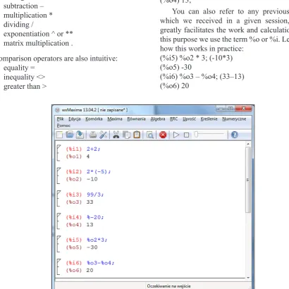
Let’s try to perform the first arithmetic opera -tions (ie, Maxima will be used as a calculator) and show the interface (Figure 1).

Note that you can refer to the previous result

with % (percent), eg: (%i4) % – 20; (33–20) (%o4) 13;

You can also refer to any previous result, which we received in a given session, which greatly facilitates the work and calculations. For this purpose we use the term %o or %i. Let us see how this works in practice:

(%i5) %o2 * 3; (-10*3) (%o5) -30

(%i6) %o3 – %o4; (33–13) (%o6) 20

(3)

46

To receive a number in decimal form, use the

function float, here is an example: (%i1) float(2/7);

(%o1) 0.28571428571429

Numerical calculations in Maxima can be

performed with any precision, the command fpprec: n will be performed with an accuracy

of n-significant digits (standard setting fpprec:

16). We can also change the accuracy of the dis-played results by typing fpprintprec: n, here is an example:

(%i1) float(23/112);

(%o1) 0.20535714285714

(%i2) fpprintprec:4$ (%i3) float(23/1121);

(%o3) 0.021

Maxima handles well with large numbers and is better than the calculator. Let us try to calculate the 2128_{and 30! Factorial operation is very}

dif-ficult to imagine, especially for high school stu -dents and ordinary calculators cannot handle such large numbers, Maxima by calculating “the facto-rial of any value” helps you to realize how much

the number is changing under its influence, which

greatly helps to develop student’s imagination. To do this in Maxima, we write:

(%i1) 2 ^ 128;

(%o1) 340282366920938463463374607431768 211456

(%i2) 30!;

(%o2) 265252859812191058636308480000000

Operator ‘ (apostrophe)

Operator ‘ prohibits the calculation of the val -ue of its argument.

Example:

(%i1) diff(sin(x),x) (%o1) cos(x) (%i2) ’diff(sin(x),x); (%o2) (sin(x))

Symbolic calculations are very good and useful, as during subsequent operations the computer does not make the mistake associ-ated with an approximation of the number.

Nested mathematical operations are often so

complicated that it is impossible to estimate it’s value. Then you can ask the program to give the approximate result of the calculation. To get the value of the expression we place the comma after it and call the command number. It requires the return of the approximate value of the

expression which is located before the comma. So far, Maxima was used as a better class of

calcula-tor. Now we will present what is beyond the reach

of a calculator.

EXPRESSIONS

The program Maxima is possible to declare algebraic expressions. You can save even the most complex expression-patterns. These ex-pressions can be freely converted, and you can

find their values at certain, fixed parameter val -ues . Maxima has many features that allow modi-fying, simplifying and developing expressions and these are the main problems of students from secondary schools. Thanks to Maxima, they may check their thinking because Maxi-ma allows you to control the partial results and calculations and all the results are displayed in symbolic form which enables precise analysis of reasoning. Let us present selected functions on algebraic expressions:

• ev(expression,condition) – modifies the ex -pression based on a condition,

• subst(b,a,expression) – after the command variable a in the expression will be replaced by variable b,

• expand(expression) – develops algebraic ex-pressions,

• ratsimp(expression) – simplifies algebraic ex -pressions,

• radcan(expression) – simplifies expression,

• factor(expression) – decomposes expression factors,

• trigexpand(expression) – develops trigono-metric expression,

• trigreduce(expression), trigsimp(expression) –

simplifies trigonometric expression

• rectform – shows the expression in the form A + B i.

• polarform – shows the complex expression in the polar form re iθ

• logcontact – simplifies the expression such as

log x + b log y. Example:

(%i1) expand((b+c)^5); // expands the expression

in brackets

(%o1) c5_+5*b*c4_+10*b2_*c3_+10*b3_*c2_+5*b4_*c+b5

Now we will factorize the expression by enter

(4)

47 DIFFERENTIATION AND INTEGRATION

The most important command to derive is diff (f (x), x); it requires the variable as the second ar-gument at which the function f(x) is differentiated and can be used to calculate the partial

deriva-tives. Diff command can have a third argument, defining the degree of derivative. These are se -lected features of the Maxima for the differential and integral calculus:

f(n)_{(x) – diff(f(x),x,n)}

• expand(expression) – develops algebraic expressions, • ratsimp(expression) – simplifies algebraic expressions, • radcan(expression) – simplifies expression,

• trigexpand(expression) – develops trigonometric expression,

• trigreduce(expression), trigsimp(expression) – simplifies trigonometric expression • rectform – shows the expression in the form A + B i.

• logcontact – simplifies the expression such as log x + b log y. Example:

(%i1) expand((b+c)^5); // expands the expression in brackets (%o1) c5_+5*b*c4_+10*b2_*c3_+10*b3_*c2_+5*b4_*c+b5

Now we will factorize the expression by enter the command: (%i2) factor(%);

(%o2) (c+b)5

4. Differentiation and integration

The most important command to derive is diff (f (x), x); it requires as the second argument the variable at which the function f(x) is differentiated and can be used to calculate the partial derivatives. Diff command can have a third argument, defining the degree of derivative. This are selected features of the Maxima for the differential and integral calculus:

f(n)_{(x) - diff(f(x),x,n)}

∫ f(𝑥𝑥)𝑑𝑑𝑥𝑥- integrate(f(x),x)

∫ f (𝑥𝑥)𝑑𝑑𝑥𝑥_𝑎𝑎𝑏𝑏 − integrate(f(x),x,a,b) or romberg(f(x),x,a,b) (calculate the integral numerically)

𝜕𝜕𝜕𝜕

𝜕𝜕𝜕𝜕 - diff(f(x,y),x)

𝜕𝜕𝜕𝜕

𝜕𝜕𝜕𝜕 - diff(f(x,y),y)

𝜕𝜕2𝜕𝜕

𝜕𝜕𝜕𝜕2 - diff(f(x,y),x,2)

𝜕𝜕2_𝜕𝜕

𝜕𝜕𝜕𝜕2 - diff(f(x,y),y,2)

𝜕𝜕𝑘𝑘+𝑛𝑛_𝜕𝜕

𝜕𝜕𝜕𝜕𝑘𝑘_{𝜕𝜕𝜕𝜕}𝑛𝑛 - diff(f(x,y),x,k,y,n) – integrate(f(x),x)

• expand(expression) – develops algebraic expressions, • ratsimp(expression) – simplifies algebraic expressions, • radcan(expression) – simplifies expression,

• trigreduce(expression), trigsimp(expression) – simplifies trigonometric expression • rectform – shows the expression in the form A + B i.

(%o2) (c+b)5

𝜕𝜕𝜕𝜕

𝜕𝜕𝜕𝜕 - diff(f(x,y),x)

𝜕𝜕𝜕𝜕

𝜕𝜕𝜕𝜕 - diff(f(x,y),y)

𝜕𝜕2𝜕𝜕

𝜕𝜕𝜕𝜕2 - diff(f(x,y),x,2)

𝜕𝜕2_𝜕𝜕

𝜕𝜕𝜕𝜕2 - diff(f(x,y),y,2)

𝜕𝜕𝜕𝜕𝑘𝑘_{𝜕𝜕𝜕𝜕}𝑛𝑛 - diff(f(x,y),x,k,y,n)

– integrate(f(x),x,a,b) or romberg(f(x), x,a,b) (calculate the integral numerically)

• expand(expression) – develops algebraic expressions,

• ratsimp(expression) – simplifies algebraic expressions,

• trigreduce(expression), trigsimp(expression) – simplifies trigonometric expression

(%o2) (c+b)5

∫ f(𝑥𝑥)𝑑𝑑𝑥𝑥 - integrate(f(x),x)

𝜕𝜕𝜕𝜕

𝜕𝜕𝜕𝜕 - diff(f(x,y),x)

𝜕𝜕𝜕𝜕

𝜕𝜕𝜕𝜕 - diff(f(x,y),y)

𝜕𝜕2_𝜕𝜕

𝜕𝜕𝜕𝜕2 - diff(f(x,y),x,2)

𝜕𝜕2_𝜕𝜕

𝜕𝜕𝜕𝜕2 - diff(f(x,y),y,2)

𝜕𝜕𝜕𝜕𝑘𝑘_{𝜕𝜕𝜕𝜕}𝑛𝑛 - diff(f(x,y),x,k,y,n) – diff(f(x,y),x)

(%o2) (c+b)5

𝜕𝜕𝜕𝜕

𝜕𝜕𝜕𝜕 - diff(f(x,y),x)

𝜕𝜕𝜕𝜕

𝜕𝜕𝜕𝜕 - diff(f(x,y),y)

𝜕𝜕2_𝜕𝜕

𝜕𝜕𝜕𝜕2 - diff(f(x,y),x,2)

𝜕𝜕2_𝜕𝜕

𝜕𝜕𝜕𝜕2 - diff(f(x,y),y,2)

– diff(f(x,y),y)

(%o2) (c+b)5

𝜕𝜕𝜕𝜕

𝜕𝜕𝜕𝜕 - diff(f(x,y),x)

𝜕𝜕𝜕𝜕

𝜕𝜕𝜕𝜕 - diff(f(x,y),y)

𝜕𝜕2_𝜕𝜕

𝜕𝜕𝜕𝜕2 - diff(f(x,y),x,2)

𝜕𝜕2𝜕𝜕

𝜕𝜕𝜕𝜕2 - diff(f(x,y),y,2)

𝜕𝜕𝑘𝑘+𝑛𝑛𝜕𝜕

– diff(f(x,y),x,2)

(%o2) (c+b)5

𝜕𝜕𝜕𝜕

𝜕𝜕𝜕𝜕 - diff(f(x,y),x)

𝜕𝜕𝜕𝜕

𝜕𝜕𝜕𝜕 - diff(f(x,y),y)

𝜕𝜕2_𝜕𝜕

𝜕𝜕𝜕𝜕2 - diff(f(x,y),x,2)

𝜕𝜕2𝜕𝜕

𝜕𝜕𝜕𝜕2 - diff(f(x,y),y,2)

𝜕𝜕𝑘𝑘+𝑛𝑛𝜕𝜕

– diff(f(x,y),y,2)

(%o2) (c+b)5

𝜕𝜕𝜕𝜕

𝜕𝜕𝜕𝜕 - diff(f(x,y),x)

𝜕𝜕𝜕𝜕

𝜕𝜕𝜕𝜕 - diff(f(x,y),y)

𝜕𝜕2𝜕𝜕

𝜕𝜕𝜕𝜕2 - diff(f(x,y),x,2)

𝜕𝜕2_𝜕𝜕

𝜕𝜕𝜕𝜕2 - diff(f(x,y),y,2)

𝜕𝜕𝜕𝜕𝑘𝑘_{𝜕𝜕𝜕𝜕}𝑛𝑛 - diff(f(x,y),x,k,y,n) – diff(f(x,y),x,k,y,n)

Examples:

1. Let f(x) = xx_{be the function whose derivative} we try to calculate, then we obtain:

(%i1) diff(x^x,x); (%o1) xx_*(log(x)+1)

2. Let the function be given by f(x) = Examples.

1. Let f(x) = xx_{be the function which derivative we try to calculate, then we obtain:} (%i1) diff(x^x,x);

(%o1) xx_*(log(x)+1)

2. Let the function be given by f(x) = sin (𝑥𝑥)_𝑥𝑥 . Calculation derivative of the second degree in Maxima looks as follows:

(%i1) diff(sin(x)/x,x,2);

(%o1) −sin (𝑥𝑥)_𝑥𝑥 +2sin (𝑥𝑥)_𝑥𝑥3 −2cos (𝑥𝑥)_𝑥𝑥2

3. The function be given by f(x, y) = 𝑥𝑥 ∗ 𝑦𝑦 + 𝑥𝑥_𝑦𝑦2₃. Let calculate its partial derivative: _{𝜕𝜕𝑥𝑥𝜕𝜕𝑦𝑦}𝜕𝜕2𝑓𝑓

(%i1) diff((x*y)+(x^2)/(y^3),x, 1, y, 1);

(%o1) 1 − 6𝑥𝑥_𝑦𝑦₄

To calculate the integrals both definite and indefinite we use integrate() command.

Example 1. We calculate ∫_𝑥𝑥2_{+4𝑥𝑥+13}7−2𝑥𝑥 𝑑𝑑𝑥𝑥

(%i1) integrate((7-2*x)/(x^2+4*x+13),x);

(%o1) 11₃ atan (2𝑥𝑥+4₆ ) − log (𝑥𝑥2_{+ 4𝑥𝑥 + 13)}

Each student can easily check the result by differentiating it and writing the following commands: (%i2) diff(%,x);

(%o2) 11 9∗((2𝑥𝑥+4)2₃₆ +1)−

2𝑥𝑥+4 𝑥𝑥2_{+4𝑥𝑥+13}

(%i3) ratsimp(%); // by this command we get a simplified result

(%o3) −_𝑥𝑥₂_{+4𝑥𝑥+13}2𝑥𝑥−7

Example 2. Let calculate the definite integral ∫ 𝑒𝑒∞ −𝑥𝑥2_{𝑑𝑑𝑥𝑥}

0 by writng command integrate(expression, variable, lower limit, upper limit):

(%i1) integrate(exp(-x*x),x,0,inf);

(%o1) √𝜋𝜋₂

Expressions can be calculated numerically by using the float(expression) command, continuing the previous example, we get:

(%i2) float(%);

(%o2) 0.88622692545276

. Calculation derivative of the second degree in Maxima looks as follows:

(%o1) – Examples.

(%o1) xx_*(log(x)+1)

3. The function be given by f(x, y) = 𝑥𝑥 ∗ 𝑦𝑦 + 𝑥𝑥_𝑦𝑦23. Let calculate its partial derivative:

𝜕𝜕2_𝑓𝑓

𝜕𝜕𝑥𝑥𝜕𝜕𝑦𝑦 (%i1) diff((x*y)+(x^2)/(y^3),x, 1, y, 1);

(%o1) 1 − 6𝑥𝑥_𝑦𝑦4

(%i1) integrate((7-2*x)/(x^2+4*x+13),x);

(%o1) 11₃ atan (2𝑥𝑥+4₆ ) − log (𝑥𝑥2_{+ 4𝑥𝑥 + 13)}

(%o2) 11 9∗((2𝑥𝑥+4)2₃₆ +1)−

2𝑥𝑥+4 𝑥𝑥2_{+4𝑥𝑥+13}

(%o3) −_𝑥𝑥₂_{+4𝑥𝑥+13}2𝑥𝑥−7

0 by writng command integrate(expression, variable, lower limit, upper limit):

(%o1) √𝜋𝜋₂

(%i2) float(%);

(%o2) 0.88622692545276 3. The function be given by f(x, y) =

Examples.

(%o1) xx_*(log(x)+1)

(%o1) −sin (𝑥𝑥)_𝑥𝑥 +2sin (𝑥𝑥)_𝑥𝑥3 −

2cos (𝑥𝑥) 𝑥𝑥2

3. The function be given by f(x, y) = 𝑥𝑥 ∗ 𝑦𝑦 + 𝑥𝑥_𝑦𝑦23. Let calculate its partial derivative: 𝜕𝜕 2_𝑓𝑓

𝜕𝜕𝑥𝑥𝜕𝜕𝑦𝑦 (%i1) diff((x*y)+(x^2)/(y^3),x, 1, y, 1);

(%o1) 1 − 6𝑥𝑥_𝑦𝑦4

(%i1) integrate((7-2*x)/(x^2+4*x+13),x);

(%o1) 11₃ atan (2𝑥𝑥+4₆ ) − log (𝑥𝑥2_{+ 4𝑥𝑥 + 13)}

(%o2) 11 9∗((2𝑥𝑥+4)2₃₆ +1)−

2𝑥𝑥+4 𝑥𝑥2_{+4𝑥𝑥+13}

(%o3) −_𝑥𝑥2_{+4𝑥𝑥+13}2𝑥𝑥−7

Example 2. Let calculate the definite integral ∫ 𝑒𝑒₀∞ −𝑥𝑥2𝑑𝑑𝑥𝑥 by writng command integrate(expression, variable, lower limit, upper limit):

(%o1) √𝜋𝜋₂

(%i2) float(%);

(%o2) 0.88622692545276

. Let calculate its partial derivative:

(%i1) diff((x*y)+(x^2)/(y^3),x, 1, y, 1);

(%o1) Examples.

(%o1) xx_*(log(x)+1)

3. The function be given by f(x, y) = 𝑥𝑥 ∗ 𝑦𝑦 + 𝑥𝑥_𝑦𝑦23. Let calculate its partial derivative: 𝜕𝜕2_𝑓𝑓 𝜕𝜕𝑥𝑥𝜕𝜕𝑦𝑦

(%i1) diff((x*y)+(x^2)/(y^3),x, 1, y, 1);

(%o1) 1 − 6𝑥𝑥_𝑦𝑦4

(%i1) integrate((7-2*x)/(x^2+4*x+13),x);

(%o1) 11₃ atan (2𝑥𝑥+4₆ ) − log (𝑥𝑥2_{+ 4𝑥𝑥 + 13)}

(%o2) 11

9∗((2𝑥𝑥+4)2₃₆ +1)− 2𝑥𝑥+4 𝑥𝑥2_{+4𝑥𝑥+13}

(%o3) −_𝑥𝑥₂_{+4𝑥𝑥+13}2𝑥𝑥−7

0 by writng command integrate(expression,

variable, lower limit, upper limit): (%i1) integrate(exp(-x*x),x,0,inf);

(%o1) √𝜋𝜋₂

(%i2) float(%);

(%o2) 0.88622692545276

To calculate the integrals both definite and in

-definite we use integrate() command.

Example 1. We calculate Examples.

(%o1) xx_*(log(x)+1)

(%o1) −sin (𝑥𝑥)_𝑥𝑥 +2sin (𝑥𝑥)_𝑥𝑥₃ −2cos (𝑥𝑥)_𝑥𝑥₂

3. The function be given by f(x, y) = 𝑥𝑥 ∗ 𝑦𝑦 + _𝑦𝑦𝑥𝑥23. Let calculate its partial derivative: 𝜕𝜕 2_𝑓𝑓 𝜕𝜕𝑥𝑥𝜕𝜕𝑦𝑦

(%i1) diff((x*y)+(x^2)/(y^3),x, 1, y, 1);

(%o1) 1 − 6𝑥𝑥_𝑦𝑦4

(%i1) integrate((7-2*x)/(x^2+4*x+13),x);

(%o1) 11₃ atan (2𝑥𝑥+4₆ ) − log (𝑥𝑥2_{+ 4𝑥𝑥 + 13)}

(%o2) 11

9∗((2𝑥𝑥+4)2₃₆ +1)− 2𝑥𝑥+4 𝑥𝑥2_{+4𝑥𝑥+13}

(%o3) −_𝑥𝑥2_{+4𝑥𝑥+13}2𝑥𝑥−7

(%o1) √𝜋𝜋₂

(%i2) float(%);

(%o2) 0.88622692545276

(%i1) integrate((7-2*x)/(x^2+4*x+13),x);

(%o1) Examples.

(%o1) xx_*(log(x)+1)

3. The function be given by f(x, y) = 𝑥𝑥 ∗ 𝑦𝑦 + 𝑥𝑥_𝑦𝑦23. Let calculate its partial derivative: 𝜕𝜕2_𝑓𝑓 𝜕𝜕𝑥𝑥𝜕𝜕𝑦𝑦

(%i1) diff((x*y)+(x^2)/(y^3),x, 1, y, 1);

(%o1) 1 − 6𝑥𝑥_𝑦𝑦4

(%i1) integrate((7-2*x)/(x^2+4*x+13),x);

(%o1) 11₃ atan (2𝑥𝑥+4₆ ) − log (𝑥𝑥2_{+ 4𝑥𝑥 + 13)}

(%o2) 11

9∗((2𝑥𝑥+4)2₃₆ +1)− 2𝑥𝑥+4 𝑥𝑥2_{+4𝑥𝑥+13}

(%o3) −_𝑥𝑥2_{+4𝑥𝑥+13}2𝑥𝑥−7

(%o1) √𝜋𝜋₂

(%i2) float(%);

(%o2) 0.88622692545276

Each student can easily check the result by differentiating it and writing the following com-mands:

(%i2) diff(%,x); (%o2)

Examples.

(%o1) xx_*(log(x)+1)

(%i1) diff((x*y)+(x^2)/(y^3),x, 1, y, 1);

(%o1) 1 − 6𝑥𝑥_𝑦𝑦₄

(%i1) integrate((7-2*x)/(x^2+4*x+13),x);

(%o1) 11₃ atan (2𝑥𝑥+4₆ ) − log (𝑥𝑥2_{+ 4𝑥𝑥 + 13)}

(%o2) 11

9∗((2𝑥𝑥+4)2₃₆ +1)− 2𝑥𝑥+4 𝑥𝑥2_{+4𝑥𝑥+13}

(%o3) −_𝑥𝑥₂_{+4𝑥𝑥+13}2𝑥𝑥−7

(%o1) √𝜋𝜋₂

(%i2) float(%);

(%o2) 0.88622692545276

(%o3) – Examples.

(%o1) xx_*(log(x)+1)

(%o1) −sin (𝑥𝑥)_𝑥𝑥 +2sin (𝑥𝑥)_𝑥𝑥₃ −2cos (𝑥𝑥)_𝑥𝑥₂

(%i1) diff((x*y)+(x^2)/(y^3),x, 1, y, 1);

(%o1) 1 − 6𝑥𝑥_𝑦𝑦₄

(%i1) integrate((7-2*x)/(x^2+4*x+13),x);

(%o1) 11₃ atan (2𝑥𝑥+4₆ ) − log (𝑥𝑥2_{+ 4𝑥𝑥 + 13)}

(%o2) 11

9∗((2𝑥𝑥+4)2₃₆ +1)− 2𝑥𝑥+4 𝑥𝑥2_{+4𝑥𝑥+13}

(%o3) −_𝑥𝑥₂_{+4𝑥𝑥+13}2𝑥𝑥−7

(%o1) √𝜋𝜋₂

(%i2) float(%);

(%o2) 0.88622692545276

Example 2. Let calculate the definite integral

Examples.

(%o1) xx_*(log(x)+1)

(%i1) diff((x*y)+(x^2)/(y^3),x, 1, y, 1);

(%o1) 1 − 6𝑥𝑥_𝑦𝑦₄

(%i1) integrate((7-2*x)/(x^2+4*x+13),x);

(%o1) 11₃ atan (2𝑥𝑥+4₆ ) − log (𝑥𝑥2_{+ 4𝑥𝑥 + 13)}

(%o2) 11

9∗((2𝑥𝑥+4)2₃₆ +1)− 2𝑥𝑥+4 𝑥𝑥2_{+4𝑥𝑥+13}

(%o3) −_𝑥𝑥₂_{+4𝑥𝑥+13}2𝑥𝑥−7

(%o1) √𝜋𝜋₂

(%i2) float(%);

(%o2) 0.88622692545276

by writing command integrate(expres-sion, variable, lower limit, upper limit):

(%i1) integrate(exp(-x*x),x,0,inf); (%o1)

Examples.

(%o1) xx_*(log(x)+1)

3. The function be given by f(x, y) = 𝑥𝑥 ∗ 𝑦𝑦 + 𝑥𝑥_𝑦𝑦23. Let calculate its partial derivative:

𝜕𝜕2_𝑓𝑓

𝜕𝜕𝑥𝑥𝜕𝜕𝑦𝑦

(%i1) diff((x*y)+(x^2)/(y^3),x, 1, y, 1);

(%o1) 1 − 6𝑥𝑥_𝑦𝑦4

(%i1) integrate((7-2*x)/(x^2+4*x+13),x);

(%o1) 11₃ atan (2𝑥𝑥+4₆ ) − log (𝑥𝑥2_{+ 4𝑥𝑥 + 13)}

(%o2) 11

9∗((2𝑥𝑥+4)2₃₆ +1)− 2𝑥𝑥+4 𝑥𝑥2_{+4𝑥𝑥+13}

(%o3) −_𝑥𝑥2_{+4𝑥𝑥+13}2𝑥𝑥−7

(%o1) √𝜋𝜋₂

(%i2) float(%);

(%o2) 0.88622692545276

Expressions can be calculated numerically by

using the float(expression) command, continuing

the previous example, we get:

(%i2) float(%);

(%o2) 0.88622692545276

The function that performs the integration in a numerical way is romberg. The Romberg () and integrate () handles well with multiple integrals (not only with the constant limits), which will surely be useful for students during calculating

fields, the volumes of solids and their surfaces. In

addition, anyone can do two or three-dimensional graphs, (we will explain it in chapter 9), this in combination with symbolic calculations made in Maxim actively growing and developing spatial imagination. We calculate:

The function that performs the integration in a numerical way is romberg. The Romberg () and integrate () handles well with multiple integrals (not only with the constant limits), which will surely be useful for students during calculating fields, the volumes of solids and their surfaces. In addition, anyone can do two or three-dimensional graphs, (we will explain it in chapter 9), this in combination with symbolic calculations made in Maxim actively growing and developing spatial imagination. We calculate: ∫ ∫ _𝑦𝑦𝑥𝑥2𝑑𝑑𝑑𝑑𝑑𝑑𝑑𝑑

6 4 2 1

(%i1) g(x,y):=x/(y^2);

(%i2) romberg(romberg(g(x,y),y,4,6),x,1,2); (%o2) 0.12500002874223

5. Systems of equations

Some useful functions for solving equations and systems of equations:

• solve (equation, variable) - solves the equation in the set of complex numbers, • linsolve ([equations], [variables]) - solves a linear system of equations,

• algsys ([equations], [variables]) - solves algebraic system equations in the set of complex numbers, if you want to receive solution in the real numbers , first you should write the following command: realonly: true,

• find_root (f (x), x, a, b) – this command find (through the approximation) zeros of the function f in the interval [a, b] (notice that f (a), f (b) should have different signs).

For example, to find a solution to the system of equations : {9𝑑𝑑 − 8𝑑𝑑 = 4_{7𝑑𝑑 + 2𝑑𝑑 = 3}we write:

(%i1) r1: 9 ∗ 𝑑𝑑 − 8 ∗ 𝑑𝑑 = 4;

(%o1) 9𝑑𝑑 − 8𝑑𝑑 = 4

(%i2) r2: 7 ∗ 𝑑𝑑 + 2 ∗ 𝑑𝑑 = 3;

(%o2) 7𝑑𝑑 + 2𝑑𝑑 = 3

(%i3) s:solve([r1,r2],[x,y]); (%o3) [[x=16/37,y=-1/74]] Checking the solution.

The following command substitute the result into to both equations. The subst() command put the expression in the first argument into the expression the second argument

(%i4) [subst(s,r1),subst(s,r2)]; (%o4) [4=4,3=3]

Solutions do not have to be a real. For equation x4_{-1 = 0, we obtain:} (%i1) solve(x^4-1);

(%o1) [x=%i,x=-1,x=-%i,x=1]

Functions realroots (W), realroots (W, accuracy) find by bisection method all real roots of a polynomial. Polynomial coefficients must be rational numbers. The second parameter defines the accuracy with which the root is searched- default is 10-7_{. In addition, each student can calculate roots}

(%i1) g(x,y):=x/(y^2);

SYSTEMS OF EQUATIONS

• solve (equation, variable) – solves the equa-tion in the set of complex numbers,

• linsolve ([equations], [variables]) – solves a linear system of equations,

• algsys ([equations], [variables]) – solves alge-braic system equations in the set of complex numbers, if you want to receive solution in the

real numbers , first you should write the fol -lowing command: realonly: true,

• find_root (f (x), x, a, b) – this command find

(through the approximation) zeros of the func-tion f in the interval [a, b ] (notice that f (a), f (b) should have different signs).

For example, to find a solution to the system

of equations

The function that performs the integration in a numerical way is romberg. The Romberg () and integrate () handles well with multiple integrals (not only with the constant limits), which will surely be useful for students during calculating fields, the volumes of solids and their surfaces. In addition, anyone can do two or three-dimensional graphs, (we will explain it in chapter 9), this in combination with symbolic calculations made in Maxim actively growing and developing spatial imagination. We calculate: ∫ ∫₁2 ₄6_𝑦𝑦𝑥𝑥2𝑑𝑑𝑑𝑑𝑑𝑑𝑑𝑑

(%i1) g(x,y):=x/(y^2);

• solve (equation, variable) - solves the equation in the set of complex numbers, • linsolve ([equations], [variables]) - solves a linear system of equations,

(%i1) r1: 9 ∗ 𝑑𝑑 − 8 ∗ 𝑑𝑑 = 4;

(%o1) 9𝑑𝑑 − 8𝑑𝑑 = 4

(%i2) r2: 7 ∗ 𝑑𝑑 + 2 ∗ 𝑑𝑑 = 3;

(%o2) 7𝑑𝑑 + 2𝑑𝑑 = 3

(%o1) [x=%i,x=-1,x=-%i,x=1]

we write: (%i1) r1:

6 4 2 1

(%i1) g(x,y):=x/(y^2);

• solve (equation, variable) - solves the equation in the set of complex numbers,

• linsolve ([equations], [variables]) - solves a linear system of equations,

(%i1) r1: 9 ∗ 𝑑𝑑 − 8 ∗ 𝑑𝑑 = 4;

(%o1) 9𝑑𝑑 − 8𝑑𝑑 = 4

(%i2) r2: 7 ∗ 𝑑𝑑 + 2 ∗ 𝑑𝑑 = 3;

(%o2) 7𝑑𝑑 + 2𝑑𝑑 = 3

(%o1) [x=%i,x=-1,x=-%i,x=1]

; (%o1)

The function that performs the integration in a numerical way is romberg. The Romberg () and integrate () handles well with multiple integrals (not only with the constant limits), which will surely be useful for students during calculating fields, the volumes of solids and their surfaces. In addition, anyone can do two or three-dimensional graphs, (we will explain it in chapter 9), this in combination with symbolic calculations made in Maxim actively growing and developing spatial imagination. We calculate: ∫ ∫₁2 ₄6_𝑦𝑦𝑥𝑥2𝑑𝑑𝑑𝑑𝑑𝑑𝑑𝑑

(%i1) g(x,y):=x/(y^2);

(%i1) r1: 9 ∗ 𝑑𝑑 − 8 ∗ 𝑑𝑑 = 4;

(%o1) 9𝑑𝑑 − 8𝑑𝑑 = 4

(%i2) r2: 7 ∗ 𝑑𝑑 + 2 ∗ 𝑑𝑑 = 3;

(%o2) 7𝑑𝑑 + 2𝑑𝑑 = 3

(%o1) [x=%i,x=-1,x=-%i,x=1]

(%i2) r2:

6 4 2 1

(%i1) g(x,y):=x/(y^2);

(%i1) r1: 9 ∗ 𝑑𝑑 − 8 ∗ 𝑑𝑑 = 4;

(%o1) 9𝑑𝑑 − 8𝑑𝑑 = 4

(%i2) r2: 7 ∗ 𝑑𝑑 + 2 ∗ 𝑑𝑑 = 3;

(%o2) 7𝑑𝑑 + 2𝑑𝑑 = 3

(%o1) [x=%i,x=-1,x=-%i,x=1]

; (%o2)

6 4 2 1

(%i1) g(x,y):=x/(y^2);

(%i1) r1: 9 ∗ 𝑑𝑑 − 8 ∗ 𝑑𝑑 = 4;

(%o1) 9𝑑𝑑 − 8𝑑𝑑 = 4

(%i2) r2: 7 ∗ 𝑑𝑑 + 2 ∗ 𝑑𝑑 = 3;

(%o2) 7𝑑𝑑 + 2𝑑𝑑 = 3

(%o1) [x=%i,x=-1,x=-%i,x=1]

(5)

48

(%i3) s:solve([r1,r2], [x,y]);

(%o3) [[x=16/37, y=-1/74]]

Checking the solution

The following command substitute the result into to both equations. The subst() command put

the expression in the first argument into the ex -pression the second argument

Solutions do not have to be a real. For equa-tion x4_{-1 = 0, we obtain:}

(%i1) solve(x^4-1);

(%o1) [x=%i,x=-1,x=-%i,x=1]

Functions realroots (W), realroots (W,

accu-racy) find by bisection method all real roots of a polynomial. Polynomial coefficients must be ra

-tional numbers. The second parameter defines the

accuracy with which the root is searched- default is 10-7_{. In addition, each student can calculate} roots e.g. quadratic equation (with parameters a, b, c: ax2_{+ bx + c = 0), and thus verify that the} formulas learned in school are rely true, and they are zeros above quadratic function. Additionally, you can also check the correctness of Viete’s for-mulas, which improve memorization and provide impetus for deepening self-knowledge.

DIFFERENTIAL EQUATIONS

The function that solves ordinary differential

equations of the first and second order is ode2

(eqn, zvar, nvar), where zvar is the dependent variable and nvar is the independent variable. To solve the differential equation we will use the

operator: ‘diff – which introduces a symbol of the

derivative and does not perform differentiation, but prepare derivative which later is part of the differential equation.

For example, we solve the differential equa-tion

eg. quadratic equation (with parameters a, b, c: ax2_{+ bx + c = 0), and thus verify that the formulas} learned in school are rely true, and they are zeros above quadratic function. Additionally, you can also check the correctness of Viete'a formulas, which improves memorization and provides impetus for deepening self-knowledge.

6. Differential Equations

The function that solves ordinary differential equations of the first and second order is ode2 (eqn, zvar, nvar), where zvar is the dependent variable and nvar is the independent variable.

To solve the differential equation we will use the operator: 'diff – which introduces a symbol of the derivative and does not perform differentiation, but prepare derivative which later is part of the differential equation.

For example, we solve the differential equation 𝑑𝑑𝑑𝑑_{𝑑𝑑𝑑𝑑} = 3𝑡𝑡2_𝑦𝑦2_{− sin (𝑡𝑡)𝑦𝑦}2

(%i1) rr:'diff(y,t,1)=3*(t*y)^2-y^2*sin(t);

(%o1) 𝑑𝑑𝑑𝑑_{𝑑𝑑𝑑𝑑} = 3𝑡𝑡2_𝑦𝑦2_{− sin (𝑡𝑡)𝑦𝑦}2

(%i2) ro:ode2(rr,y,t); // solution of the differential equation (%o2) 1/y=-cos(t)-t3_{+%c //notice that %c is constant value} (%i3) rs:ic1(ro,t=0,y=1); // initial condition y(0)=1 (%o3) 1/y=-cos(t)-t3₊₂

(%i4) method; // We can ask about the type of the equation and we get: (%o4) separable // variable-separated

If Maxima can not solve a differential equation, as a result returns false. 8. Matrices

The Maxima has many functions related to matrices. Matrices are introduced to the program by using the function matrix, to perform the matrix product we use a dot (not *). The use of other features we show on an example:

If we use the function genmatrix of undefined parameter, we obtain a general matrix with elements aij.

(%i1) genmatrix(a,2,2);

(%o1) [𝑎𝑎_𝑎𝑎1,1_2,1 𝑎𝑎_𝑎𝑎1,2_2,2]

We calculate the determinant by writing the following command: (%i2) determinant(%);

(%o2) a1,1a2,2-a1,2a2,1

We can also (symbolically) designate the inverse matrix:

(%i3) invert(%o1) ; // Simplified result which we obtain by using the following function: (%i4) ratsimp(%); //then we have:

(%i1) rr:’diff(y,t,1)=3*(t*y)^2-y^2*sin(t); (%o1)

(%o1) [𝑎𝑎_𝑎𝑎1,1_2,1 𝑎𝑎_𝑎𝑎1,2_2,2]

(%o2) a1,1a2,2-a1,2a2,1

(%i2) ro:ode2(rr,y,t); // solution of the differential

equation

(%o2) 1/y=-cos(t)-t3_{+%c //notice that %c is con} -stant value

(%i3) rs:ic1(ro,t=0,y=1); // initial condition y(0)=1 (%o3) 1/y=-cos(t)-t3₊₂

(%i4) method; // We can ask about the type of the

equation and we get:

(%o4) separable // variable-separated

If Maxima cannot solve a differential equa-tion, as a result returns false.

MATRICES

The Maxima has many functions related to matrices. Matrices are introduced to the program by using the function matrix, to perform the ma-trix product we use a dot (not *). The use of other features we show on an example:

If we use the function genmatrix of undefined

parameter, we obtain a general matrix with ele-ments a_ij.

(%i1) genmatrix(a,2,2); (%o1)

(%o1) [𝑎𝑎_𝑎𝑎1,1_2,1 𝑎𝑎_𝑎𝑎1,2_2,2]

(%o2) a1,1a2,2-a1,2a2,1

We calculate the determinant by writing the following command:

(%i2) determinant(%); (%o2) a_1,1a_2,2-a_1,2a_2,1

We can also (symbolically) designate the in-verse matrix:

(%i3) invert(%o1) ; // Simplified result which we

obtain by using the following function:

(%i4) ratsimp(%); //then we have:

(%o4) (%o4) [

𝑎𝑎2,2 a1,1a2,2−a1,2a2,1

−𝑎𝑎1,2 a1,1a2,2−a1,2a2,1 −𝑎𝑎2,1

a1,1a2,2−a1,2a2,1

𝑎𝑎1,1 a1,1a2,2−a1,2a2,1

]

These symbolic calculations also make remembering easier and preserve the fundamental rights that are used by the students in all science, they also inspire to continue learning mathematics.

Although the Maxima is a symbolic algebra system also allow us for numerical operations, also with elements of linear algebra. We can calculate for example:

• the eigenvalues of the matrix A and their multiplicities - eigenvalues(A),

• rank of a matrix A - rank(A),

• eigenvalues of a square matrix A, with their multiples and their eigenvectors - eigenvectors(A),

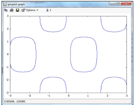
• transposition of matrix A - transpose(A) 9. Graphs

At the beginning of drawing graphs we will present and talk over some examples of functions and their parameters. Let f1(x):= (x_(x2₂−1)₊₁₎

(%i1) f1(x):=(x^2-1)/(x^2+1)$

(%i2) plot2d(f1(x),[x,-8,8]); \\ Drawing the function y:=f1(x) in the range -8 <= x <=8

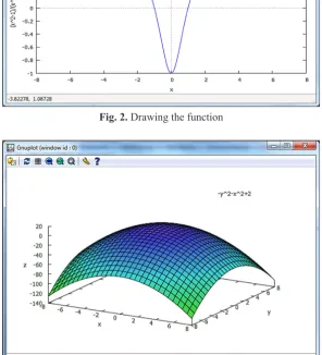
We can also do three-dimensional graphs in Maxima, here's an example: Let fc(x,y):=2-x2_-y2

(%i1) fc(x,y):=2-x^2-y^2$

(%i1) plot3d( fc(x,y), [x,-8,8], [y,-8,8]);

These symbolic calculations also make re-membering easier and preserve the fundamental rights that are used by the students in all science, they also inspire to continue learning mathematics.

Although the Maxima is a symbolic algebra system also allow us for numerical operations, also with elements of linear algebra. We can cal-culate, for example:

• the eigenvalues of the matrix A and their mul-tiplicities – eigenvalues(A),

• rank of a matrix A – rank(A),

• eigenvalues of a square matrix A, with their mul-tiples and their eigenvectors – eigenvectors(A), • transposition of matrix A – transpose(A)

GRAPHS

At the beginning of drawing graphs we will present and talk over some examples of functions and their parameters. Let f1(x):=

(%o4) [

𝑎𝑎2,2 a1,1a2,2−a1,2a2,1

−𝑎𝑎1,2 a1,1a2,2−a1,2a2,1 −𝑎𝑎2,1

a1,1a2,2−a1,2a2,1

𝑎𝑎1,1 a1,1a2,2−a1,2a2,1

]

These symbolic calculations also make remembering easier and preserve the fundamental rights that are used by the students in all science, they also inspire to continue learning mathematics.

Although the Maxima is a symbolic algebra system also allow us for numerical operations, also with elements of linear algebra. We can calculate for example:

• the eigenvalues of the matrix A and their multiplicities - eigenvalues(A),

• rank of a matrix A - rank(A),

• eigenvalues of a square matrix A, with their multiples and their eigenvectors - eigenvectors(A),

• transposition of matrix A - transpose(A)

9. Graphs

At the beginning of drawing graphs we will present and talk over some examples of functions and their parameters. Let f1(x):= (x_(x2₂−1)₊₁₎

(%i1) f1(x):=(x^2-1)/(x^2+1)$

(%i2) plot2d(f1(x),[x,-8,8]); \\ Drawing the function y:=f1(x) in the range -8 <= x <=8

We can also do three-dimensional graphs in Maxima, here's an example: Let fc(x,y):=2-x2_-y2

(%i1) fc(x,y):=2-x^2-y^2$