Coverage Problems in Sensor Networks

Coverage Problems in Sensor Networks

Dr. Srinivasa Rao Angajala

Professor,

Mekapati Rajamohan Reddy Institute of Technology & Science, Udayagiri -524226, Sri Potti Sri Ramulu Dist., A.P.,India, [email protected]

Abstract - Now a day’smost vital part of research covers on Wireless Adhoc Sensor Networks due to broad collection of prospective applications. A wireless Sensor network causes a new theoretical and challenging optimization problem. Now here we discuss one of the essential problems of coverage in sensor networks, which reflects the quality of surveillance of accurate sensor network. The conception of coverage is considered from several points of view due to a variety of sensor networks and ample sort of their applications. We inclusively present tentative outcomes and overview of future research information related to coverage of sensor networks.

Keywords - Sensor Network, Radar, Sensor scheduling, Coverage

I. I

As our personal computing era evolves into a ubiquitous computing one, there is a need for a world of fully connected devices with inexpensive wireless networks. Improvements in wireless network technology interfacing with emerging micro-sensor based on MEMs technology [2], is allowing sophisticated inexpensive sensing, storage, processing, and communication capabilities to be unobtrusively embedded into our everyday physical world. Moreover, embedded web servers [1, 3] can be used to connect the physical world of sensors and actuators to the virtual world of information utilities and services. Consequently, a flurry of research activity has recently commenced in the sensor network domain, especially in wireless ad-hoc sensor networks. Although many of the sensor technologies are not new, there are certain physical laws governing the energy requirements of performing wireless communications that have limited the feasibility of such devices in the past. Some of the benefits of the newer, more capable sensor nodes are the ability to:

 Build large-scale networks;

 Implement sophisticated protocols;

 Reduce the amount of communication (wireless) required to perform tasks by distributed and/or local precomputations;

 Implement complex power saving modes of operation depending on the environment and the state of the network.

Due to the above-mentioned advances in sensor network technology, more and more practical applications of wireless sensor networks continue to emerge. As an example, consider the millions of acres that are lost around the world, due to forest fires every year. In all fires, early warnings are critical in preventing small harmless brush fires from

becoming monstrous infernos. By deploying specialized wireless sensor nodes in strategically selected high-risk areas, the detection time for such disasters can be drastically reduced, increasing the likelihood of success in early extinguishing efforts. Also, since the nodes are self-configuring and do not need constant monitoring, the cost of such a deployment is minimal compared to the huge losses incurred in a large blaze.

In addition to the new applications, wireless sensor networks provide a viable alternative to several existing technologies. For example, large buildings contain hundreds of environmental sensors that are wired to a central air conditioning and ventilation system. The significant wiring costs limit the complexity of current environmental controls and the reconfigurability of these systems. However, replacing the hard-wired monitoring units with ad-hoc wireless sensor nodes can improve the quality and energy efficiency of the environmental system while allowing almost unlimited reconfiguration and customization in the future. In many instances, the savings in the wiring costs alone justify the use of the wireless sensor nodes.

B. Research Goal: Sensor Network Coverage

One of the fundamental issues that arise in sensor networks, in addition to location calculation, tracking, and deployment, is coverage. Due to the large variety of sensors and applications, coverage is subject to a wide range of interpretations. In general, coverage can be considered as the measure of quality of service of a sensor network. For example, in the previous fire detection sensor networks example, one may ask how well the network can observe a given area and what the chances are that a fire starting in a specific location will be detected in a given time frame. Furthermore, coverage formulations can try to find weak points in a sensor field and suggest future deployment or reconfiguration schemes for improving the overall quality of service. In most sensor networks, two seemingly contradictory, yet related viewpoints of coverage exist:

worst and best case coverage. In worst-case coverage,

time algorithm for coverage in sensor networks. We combine existing computational geometry techniques and constructs such as the Voronoi diagram, with graph theoretical algorithmic techniques. The use of Voronoi diagram, efficiently and without loss of optimality, transforms the continuous geometric problem into a discrete graph problem. Furthermore, it enables direct application of search techniques in the resulting graph representation. We also study asymptotic coverage behavior of random wireless ad-hoc networks.

C. Paper Organization

The reminder of the paper is organized as follows: In the next section we summarize the related work. In section III, we survey several key technologies that are fundamental to our study of coverage. Section IV contains a brief overview of deterministic sensor deployment and coverage. In section V, we present a formal definition of the worst (breach) and best (support) coverage and propose optimal polynomial-time algorithms for solving each case. Section VI contains a wide array of experimental results followed by a brief discussion of our future research directions and the conclusion.

II. R

W

The increasing trend in research efforts in the areas referred to as Smart Spaces or Pervasive Computing are directly related to many problems in sensor networks. Although many researchers in the sensor network area have mentioned the critical notion of coverage in the network, to our knowledge this is the first time that an algorithmic approach combined with computational geometry constructs was adopted in ad-hoc sensor networks. Also, to our knowledge, [18] was the first to identify the importance of computational geometry and Voronoi Diagrams in sensor network coverage. Reference [11] describes a general systematic method for developing an advanced sensor network for monitoring complex systems such as those found in nuclear power plants but does not present any general coverage algorithms. The Art Gallery Problem [12] deals with determining the number of observers necessary to cover an art gallery room such that every point is seen by at least one observer. It has found several applications in many domains such as the optimal antenna placement problems for wireless communication. The Art Gallery problem was solved optimally in 2D and was shown to be NP-hard in the 3D case. Reference [12] proposes heuristics for solving the 3D case using Delaunay triangulation. Sensor coverage for detecting global ocean color where sensors observe the distribution and abundance of oceanic phytoplankton [7] is approached by assembling and merging data from satellites at different orbits.

Perhaps the most related works are the attempts on coverage of an initially unknown environment for mobile robots [4, 6]. However, when the geometry of the

environment is known in advance, coverage becomes a special case of path planning [10]. Both of these problems are solved using generalized Voronoi diagrams. Radar and sonar coverage also present several related challenges. The radar and sonar netting optimization is of great importance in the networking technologies and the optimal distribution of detection and tracking in a surveillance area [15]. Based on the measured radar cross sections and the coverage diagrams for different radars, [16] proposes a method for optimally locating the radars to achieve a satisfactory surveillance area with limited radar resources.

Coverage studies to maintain connectivity have also been the focus of study. For example, [13] and [14] calculate the optimum number of base stations required to achieve the system operator's service objectives. Previously, connectivity was achieved through mobile host attachments to a base station. However, the connectivity coverage is more important in the case of ad-hoc wireless networks since the connections are peer-to-peer. Reference [9] shows the improvement in the network coverage due to the multi-hop routing features and optimizes the coverage constraint to the limited path length. Although our coverage study is aimed at ad-hoc wireless sensor networks, it is different from the above-mentioned class of problems due to our geometrical algorithmic approach

.

III. P

A. Topology of the network and Sensor Model

Generally, wireless sensor networks are targeted to the extremes of miniaturization, availability, accuracy, reliability, and power savings. This requires a networked infrastructure with small physical nodes, low power consumption, and low cost, that in turn limits communications to the immediate proximity of each node. There are several existing models of sensor behavior each with varying degrees of complexity. However, most models share one thing in common in that generally, sensing ability is directly dependant on distance. Consequently, in all our subsequent discussions, we assume that sensor coverage decreases as distance from sensors increases.

B. Enabling Technologies: Sensor Location

Technology and Algorithms

few of the sensor nodes called beacons know their coordinates in advance, either from satellite information (GPS) or pre-deployment. The reallocation scheme then relies on signal strength information embedded in the inherent radio frequency communication capabilities of the nodes in approximating neighbor distances. Each node that can hear from a minimum of three beacon neighbors can determine its own location by trilateration and become a beacon. Iterative trilaterations are then used to locate as many nodes as possible.

We have also developed heuristics to compensate for the errors in the initial beacon locations and distance information. Initial analysis and percolation simulations show that in a reasonably dense network, by having 1% or less of the nodes as initial beacons, almost all other nodes can locate themselves at the end of the location process. In our discussions of coverage algorithms, we only consider nodes that have valid location information.

C. Enabling Technology: Computational Geometry

Voronoi Diagram and Delaunay Triangulation

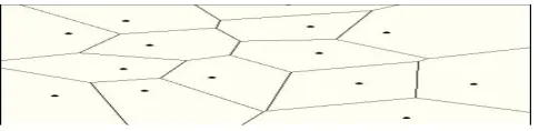
The Voronoi diagram has been re-invented, used, and studied in many domains. According to [5] it is believed that the Voronoi diagram is a fundamental construct defined by a discrete set of points. In 2D, the Voronoi diagram of a set of discrete sites (points) partitions the plane into a set of convex polygons such that all points inside a polygon are closest to only one site. This construction effectively produces polygons with edges that are equidistant from neighboring sites. Fig.1 shows an example of a Voronoi diagram for a set of randomly placed sites. Reference [5] presents a detailed survey of Voronoi diagrams and their applications. Another structure that is directly related to Voronoi diagrams is the Delaunay triangulation [8]. The Delaunay triangulation can be obtained by connecting the sites in the Voronoi diagram whose polygons share a common edge. It has been shown that among all possible triangulations, the Delaunay triangulation maximizes the smallest angle in each triangle. Also, neighborhood information can be extracted from the Delaunay triangulation since sites that are close together are connected. In fact the Delaunay triangulation can be used to find the two closest sites by considering the shortest edge in the triangulation. We use the properties of the Voronoi diagram and Delaunay triangulation to solve for best and worst case coverages.

Fig. 1 - Voronoi Diagram Of A Set Of Randomly Placed Points in a Plane

D. Implementation: Centralized vs. Distributed

Multi-hop communication is one of the main enablers in reducing power consumption in ad-hoc sensor networks. The energy required for communication between two arbitrary nodes A and B is strongly dependent on the distance d between the two nodes. More precisely, E = B

y

d where y>1 is the path loss exponent depending on the RF

environment and B is a proportionality constant describing the overhead per bit. Given this super linear relationship between energy and distance, generally using several short intermediate hops to send a bit is more energy efficient than using one longer hop. However, an incorrect conclusion would be to use an infinite number of hops over the smallest possible distances. In reality, this is impractical for two reasons:

i) The number of intermediate hops is limited by the number of nodes between A and B;

ii) The energy is not limited to the energy radiated through the antenna. There is also the energy dissipated in the radio for receiving a bit and readying a bit for retransmission.

For applications such as coverage calculations, the energy of computations per node is also a component of the energy metric. It is important to note that technology scaling will gradually reduce the processing costs, with the transmission cost remaining constant. Using compression techniques, one can reduce the number of transmitted bits, thus reducing the cost of transmission at the expense of more computation. This communication-computation trade-off is the core idea behind low energy sensor networks. From this discussion it is apparent that a good algorithm designed for wireless sensor networks will require minimal amount of communication. This is in sharp contrast with classical distributed systems [19] where the goal generally is maximizing the speed of execution. This renders the classical distributed algorithm irrelevant for developing wireless sensor networks algorithms.

The most relevant metrics in wireless networks is power. Experimental measurements indicate that communication cost in wireless ad-hoc networks is at least two orders of magnitude higher than computation costs in terms of consumed power. Note that the coverage problem is intrinsically global in the sense that, lack of knowledge of location of any single node implies that the problem may not be solved correctly. Therefore, any algorithm which aims to provide correct solution must inherently use all location data.

IV. D

C

compensate for the more critically monitored areas. An example of a uniform deterministic coverage is the grid-based sensor deployment where nodes are located on the intersection points of a grid. In this case, the problem of coverage of the sensor field reduces to the problem of coverage of one cell and its neighborhood due to the symmetric and periodic deployment scheme. An example of weighted predefined deployment is the security sensor systems used in museums. The more valuable exhibit items are equipped with more sensors to maximize the coverage of the monitoring scheme. Another deterministic deployment scheme can be found in the 3D Art Gallery Problem heuristics solutions discussed in [12]. Our proposed coverage algorithm can be used in all predefined (deterministic) deployment schemes to determine the coverage in the sensor field.

V. S

C

In many situations, deterministic deployment is neither feasible nor practical. Another deployment option is to cover the sensor field with sensors randomly distributed in the environment. The stochastic random distribution scheme can be uniform, Gaussian, Poisson or any other distribution based on the application at hand. In the simulation studies for this paper, we have generally assumed uniform sensor distribution, although our algorithm is applicable to any other deployment scheme of the sensor nodes.

A. Worst Case Coverage- Maximal Breach Path

The breach-based coverage discussed earlier can formally be stated as:

Given: A field A instrumented with sensors S where for each sensor siS, the location (xi,yi) is known; areas I and F

corresponding to initial (I) and final (F) locations of an agent.

Problem: Identify PB, the Maximal Breach Path in S,

starting in I and ending in F. PB in this case is defined as a

path through the field A, with end-points I and F and with the property that for any point p on the path PB, the distance

from p to the closest sensor is maximized. The regions I and

F are arbitrary regions determined by the task at hand and

may be located anywhere inside or outside the sensor field. Since by construction, the line segments of the Voronoi diagram maximize distance from the closest sites, the Maximal Breach Path PB, must lie on the line segments of the Voronoi diagram corresponding to the sensors in S. If any point p on the path PB deviates from Voronoi line

segments, by definition, it must be closer to at least one sensor in S. Thus, the following three steps obtain the solution to this problem:

1) Generate Voronoi diagram for S; 2) Apply graph theory abstraction;

3) Find PBusing Binary-Search and Breadth-First-Search.

The lines at the boundaries of the Voronoi diagram extend to infinity. However, since here we are dealing with a finite area A, we must clip the Voronoi diagram to the boundaries of A. Since traveling along the bounds of the sensor field also constitutes a valid path, we introduce extra edges in the Voronoi diagram corresponding to the bounds of A. In subsequent discussions, when we refer to the Voronoi diagram, we are actually referring to the bounded Voronoi diagram.

The first part of the algorithm detailed in Fig. 2 generates the Voronoi diagram corresponding to the sensors in S. The weighted, undirected graph G is constructed by creating a node for each vertex and an edge corresponding to each line segment in the Voronoi diagram. Each edge in graph G is given a weight equal to its minimum distance from the closest sensor in S. The algorithm then performs a binary search between the smallest and largest edge weights in G. In each step, breadth-first-search is used to check the existence of a path from I to F using only edges with weights that are larger than the search criteria called

breach_weight. If a path exists, breach_weight is increased

to further restrict the edges considered in the next search iteration. If a path is not found, breach_weight is lowered to relax the constraint on the search. Upon completion, the algorithm has found the Maximal Breach Path, which is the path from I to F with the highest possible weighted edges.

Generate Bounded Voronoi diagram for S with vertex set U and line segment set L.

Initialize weighted undirected graph G(V,E)

FOR each vertex uiU Create duplicate vertex viin V FOR each li(uj,uk)L

Create edge ei(vj,vk) in E

Weight(ei)=min distance from sensor siS for 1≤i≤|S| min_weight = min edge weight in G

max_weight = max edge weight in G range = (max_weight–min_weight) / 2 breach_weight = min_weight + range

WHILE (range > binary_search_tolerance)

Initialize graph G’(V’,E’) FOR each viV

Create vertex vi’in G’ FOR each eiE

IF Weight(ei)≥breach_weight Insert edge ei’in G’

range = range / 2

IF BFS(G’,I,F) is Successful

breach_weight = breach_weight + range

ELSE

breach_weight = breach_weight–range

END IF

Fig. 2 - Maximal Breach Path Algorithm

2

2 breach_weight determined in the binary search phase of the

algorithm, with at least one edge that has a weight equal to

breach_weight. The breach_weight found by the algorithm

is the minimum distance from sensors that an agent traveling on any path through the field A (from I to F) must encounter at least once. If new sensors can be deployed or existing sensors moved such that this breach_weight is decreased, then the worst-case coverage is improved.

B. Best Case Coverage- Maximal Support Path

Similar to the worst-case (breach) coverage formulation, the best-case (support) coverage can be stated as:

Given: A field A instrumented with sensors S where for

each sensor siS, the location (xi,yi) is known; areas I and F

corresponding to initial (I) and final (F) locations of the agent.

Problem: Identify PS, the path of maximal support in S,

starting in I and ending in F.

PSin this case is defined as a path through the field A, with

end-points I and F, and with the property that for any point p on the path PS, the distance from p to the closest sensor is

minimized.

Since the Delaunay triangulation produces triangles that have minimal edge lengths among all possible triangulations, PS must lie on the lines of the Delaunay

triangulation of the sensors in S. intuitively, if one tries to move in S while minimizing distance from sensors, one must attempt to travel along straight lines connecting sensor nodes. The algorithm for solving for PSis very similar to the

breach algorithm in Figure 2 with the following exceptions:

i) The Voronoi diagram is replaced by the Delaunay triangulation as the underlying geometric structure; ii) The edges in graph G are assigned weights equal to the

length of the corresponding line segments in the Delaunay triangulation;

iii) The search parameter breach_weight is replaced by the new parameter support_weight.

In this case, the maximal support path may also not be unique. However, the support_weight found in the binary search phase of the algorithm is indicative of the best-case coverage of the network. Here, support_weight is the maximum distance from the closest sensors that an agent traveling on any path through the field A (from I to F) must encounter at least once. If additional sensors can be deployed or existing sensors moved such that

support_weight is decreased, then the best-case coverage is

improved.

C. Complexity

The best known algorithms for the generation of the Voronoi diagram have O(n log n) complexities. The conversion to graphs and weight assignments can be accomplished in linear time and therefore do not add any

significant overhead to the computation. In most cases, BFS (and DFS) have O(m) complexity where m is the number

of edges in the graph. Since in realistic cases we deal with sparse networks the actual complexity is O(n) while it could be as high as O(n ). Binary search is accomplished in O(log

range) where range is usually limited. So, while the worst

case complexity of the algorithm is O(n log n), in practice the networks are sparse and the overall complexity is O(n

log n), dominated by the Voronoi procedure which has large

constant factor in its complexity

.

VI. E

R

A. Experimentation Platform - Sample Results

The coverage algorithms presented here have been implemented and used in several studies including simulations using NS (Network Simulator) and stand-alone C packages. In this section, we present a sampling of the results and try to provide an overview and analysis of the applications.

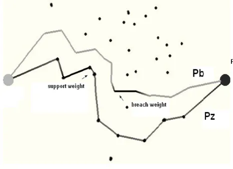
Fig. 3 shows an instance of the coverage problem where

30 sensors are deployed at random. The Maximal Breach Path (PB) and the corresponding edge with breach_weight

depicts where the breach takes place in the field. The Maximal Support Path (PS) and the corresponding edge with support_weight are also shown.

Fig. 4 shows the underlying bounded Voronoi diagram for

the same problem instance. Extra edges with 0 weight are used to connect the I and F regions to the structure so that all possible paths can be considered in the search algorithm.

Fig. 5 shows the corresponding Delaunay triangulation. In

this case, only two extra edges are introduced to connect I and F to the closest sensors in the structure.

Fig. 4 - Sensor Field With Weighted Voronoi Diagram And Maximal Breach Path

Fig. 5 - Sensor Field with Weighted Delaunay Triangulation and Maximal Support Path (PS)

B. Sensor Deployment Heuristics

The edges corresponding to breach_weight described in section V can be used as a guide for future sensor deployments. Since breach_weight corresponds to the edge in the breach path where PBis closest to the sensors,

deploying additional sensors along that edge can improve overall coverage.

Fig. 6 - Average Breach Coverage Improvement By Additional Sensor Deployment.

Fig. 6 shows the average improvement in breach coverage

when up to 4 additional sensors are introduced in the network according to the heuristic described above. Note that after each additional sensor deployment, the algorithm

was repeated to find the new breach region. The results represent average improvements over 100 random deployments. It is interesting that even after deploying 100 sensors, breach coverage can be improved by about 10% by deploying just one more sensor.

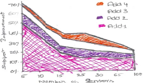
Similarly, the support_weight and the mid-point of the corresponding edge in the Delaunay triangulation can be used as a heuristic for deploying additional sensors to improve support coverage. As shown in Fig.7, on average, a 50% improvement can be achieved in support coverage by adding 1 additional sensor when 5 nodes have already been randomly deployed. After deploying 100 random sensors, on average a 10% support coverage improvement can be expected by using the heuristic to deploy one more sensor.

Fig. 7 - Average Support Coverage Improvement By Additional Sensor Deployment

C. Asymptotic Behavior

Fig. 8 - Normalized Breach (breach_weight) and Support (1-support_weight) Coverage as a Function of Number of

Sensor Nodes

Both breach and support, lower values of breach _ weight and support_weight respectively, indicate better coverage from the sensor field. Fig. 8 demonstrates the asymptotic nature of these metrics from the sensor field operator's point of view who wants to minimize breach and maximize support. Thus for clarity, the figure shows a normalized plot of breach_weight and 1-suppor t _weight as a function of the number of sensors.

Given the unit square field and using the distance based sensor model described earlier, on average, after deploying about 100 sensors, additional random sensors do not improve coverage very significantly. This asymptotic nature of breach and support coverage suggests that by analyzing a given field and selecting the proper number of sensor nodes, certain levels of coverage can be expected even if sensor deployment cannot be performed according to an exact plan.

VII. F

R

D

There is a large horizon of possibilities for future researches on this subject. The solution for obtaining a ubiquitous context is to assemble information from a combination of related services. Such information fusion is similar in intent to the related and well-researched area of sensor fusion. For the context of coverage, negotiation and resolution strategies are needed to integrate information from this stage to be used in related contexts such as tracking mobile objects in the network and handling obstacles.

In this paper, we have assumed identical sensor sensitivities where the coverage depends only on the geometrical distances from sensors. In practice, other factors influence coverage such as obstacles, environmental conditions, and noise. In addition to non-homogeneous sensors, other possible sensor models can deal with non-isotropic sensor sensitivities, where sensors have different sensitivities in different directions. The integration of multiple types of sensors such as seismic, acoustic, optical, etc. in one network platform and the study of the overall coverage of the system also presents several interesting challenges.

VIII. C

Several interpretations and formulations of coverage in wireless ad-hoc sensor networks were presented. An optimal polynomial time algorithm that uses graph theoretic and computational geometry constructs was proposed for solving for best and worst case coverages. Experimental results show several applications of the theoretic coverage formulations and algorithms specifically for solving for Maximal Breach Path, Maximal Support Path, and additional sensor deployment heuristics to improve coverage, and stochastic field coverage.

R

[1] D. Tennenhouse, Proactive Computing, Communications of the ACM, vol.43, pp. 43-50, May 2000.

[2] G.J. Pottie, W.J. Kaiser, “Wireless Integrated Network Sensors,”

Communications of the ACM, vol.43, pp. 51-58, May 2000.

[3] G. Borriello, R. Want, “Embedded Computation Meets The World Wide Web,”Communications of the ACM, vol.43, pp. 59-66, May 2000.

[4] G.S. Sukhatme, M.J. Mataric,“Embedding Robots Into The Internet,” Communications of the ACM, vol.43, pp. 67-73, May 2000.

[5] F. Aurenhammer,“Voronoi Diagrams–A Survey Of A Fundamental Geometric Data Structure,”ACM Computing Surveys 23, pp. 345-405, 1991.

[6] Z.J. Butler, A.A. Rizzi, R.L. Hollis,“Contact Sensor-Based Coverage Of Rectilinear Environments,” IEEE International Symposium on Intelligent Control Intelligent Systems and Semiotics, pp. 266-271, Sept. 1999.

[7] W.W. Gregg, W.E. Esaias, G.C. Feldman, R. Frouin, S.B. Hooker, C.R. McClain, R.H. Woodward,“Coverage Opportunities For Global Ocean Color In A Multimission Era”, IEEE Transactions on Geoscience and Remote Sensing, vol.36, pp. 1620-7, Sept. 1998 [8] K. Mulmuley, Computational Geometry: An Introduction Through

Randomized Algorithms, Prentice-Hall, 1994.

[9] Z.J. Haas, “On The Relaying Capability Of The Reconfigurable

Wireless Networks,” IEEE 47th Vehicular Technology

Conference,vol.2, pp. 1148-52, May 1997.

[10] C.W. Kang, M.W. Golay,“An Integrated Method For Comprehensive Sensor Network Developement In Complex Power Plant Systems,” Reliability Engineering & System Safety, vol.67, pp. 17-27, Jan. 2000. [11] M. Marengoni, B.A. Draper, A. Hanson, R.A. Sitaraman,“System To Place Observers On A Polyhedral Terrain In Polynomial Time,” Image and Vision Computing, vol.18, pp. 773-80, Dec. 1996. [12] A. Molina, G.E. Athanasiadou, A.R. Nix,“The Automatic Location Of

Base-Stations For Optimised Cellular Coverage: A New

Combinatorial Approach,” IEEE 49th Vehicular Technology

Conference, vol.1, pp. 606-10, May 1999.

[13] Seapahn Meguerdichian, Farinaz Koushanfar, iodrag Potkonjak, Mani B. Srivastav,” Coverage Problems in Wireless Sensor Networks: Designs and Analysis.” Dept. of Computer Science & Engineering University of Minnesota.