Efficient decoding algorithm for convolution coding used in communication systems

(1)

Int. J. Adv. Res. Sci. Technol. Volume 4, Issue 1, 2015, pp.271-275.

International Journal of Advanced Research in

Science and Technology

journal homepage: www.ijarst.com

ISSN 2319 – 1783 (Print)

ISSN 2320 – 1126 (Online)

Efficient decoding algorithm for convolution coding used in communication systems

Bh. Sirisha* and B. Venugopal

Department of ECE, Koushik college of Engg.,Visakapatnam, Andhra Pradesh, India.

*Corresponding Author’s Email: [email protected]

A R T I C L E I N F O A B S T R A C T

Article history:

Received Accepted Available online

20 Nov. 2014 11 Dec. 2014 20 Jan. 2015

Convolution encoder and Viterbi decoder are the basic and important blocks in any Code Division Multiple Accesses (CDMA). They are widely used in communication system due to their error correcting capability but the performance degrades with variable constraint length. In this context to have detail analysis. The best way of decoding against random errors is to compute the received sequence with every possible code sequence. This is called maximum likelihood (ML) decoding. The criterion for deciding between two paths is to select the one having the smaller metric. The rule maximizes the probability of a correct decision. The Viterbi algorithm occupies large memory and computational resources. To address this problem Proposed Viterbi Algorithm is introduced. The Proposed Viterbi decoder functionally is same as the previous Viterbi decoder but it reduces memory and the hardware resources. The proposed block diagram checks every node for path metric value and eliminates the path that is found if it is not having minimum distance. This paper deals with the implementation of convolution encoder and Viterbi decoder for fixed constraint length. It uses a fixed constraint length of 8 bits for ½ code rate. By analysing the Viterbi algorithm it is seen that our algorithm has a better error rate for ½ code rates than 1/3. The reduced bit error rate with increasing constraint length shows an increase in efficiency and better utilization of resources as bandwidth and power.

Keywords:

weight Matrix (WM),

Rise over Therml noise (RoT), High Speed Downlink Packet Access (HSDPA).

Introduction:

The Viterbi Algorithm was developed by Andrew J. Viterbi and first published in the IEEE transactions journal on Information theory in 1967. It was first proposed as a solution to the decoding of convolutional codes .The VA is often looked upon as minimizing the error probability by comparing the likelihoods of a set of possible state transitions that can occur, and deciding which of these has the highest probability of occurrence. It is a maximum likelihood decoding algorithm for convolutional codes. This algorithm provides a method of finding the branch in the trellis diagram that has the highest probability of matching the actual transmitted sequence of bits. Since being discovered, it has become one of the most popular algorithms in use for convolutional decoding. Apart from being an efficient and robust error detection code, it has the advantage of having a fixed decoding time. This makes it suitable for hardware implementation.

The Viterbi decoding algorithm is a decoding process for convolutional codes for memory-less

channel. Below figure depicts the normal flow of information over a noisy channel. For the purpose of error recovery, the encoder adds redundant information to the original Information , and the output is transmitted through a channel. Input at receiver end (r) is the information with redundancy and possibly, noise. The receiver tries to extract the original information through a decoding algorithm and generates an estimate (e). A decoding algorithm that maximizes the probability p(r|e) is a maximum likelihood (ML) algorithm.

(2)

The channel encoder accepts the message bits and adds redundancy according to a prescribed rule, there by producing encoded data at a higher bit rate. The channel decoder exploits the redundancy to decide which message bit was actually transmitted. The combined goal of the channel encoder and decoder is to minimize the effect of channel noise. That is the number of errors between the channel encoder input and the channel decoder output is minimized.

The addition of redundancy in the coded messages implies the need for increase in transmission bandwidth. The use of coding adds complexity to the system, especially for the implementation of decoding operations in the receiver. Thus, the design trade-offs in the use of error control coding to achieve acceptable error performance must include considerations of bandwidth and system complexity.

These codes have been classified into Block codes and Convolution codes. Block codes are further classified into Linear block codes and Cyclic codes Convolution codes follow Tree diagram, State diagram andTrellis diagram.

Convolutional Encoding Mechanism:

Data is coded by using a convolutional encoder. It consists of a series of shift registers and an associated combinatorial logic. The combinatorial logic is usually a series of exclusive-or gates. The conventional encoder ½ K=7, (171,133) is used for the purpose of this project. The octal numbers 171 and 133 when represented in binary form correspond to the connection of the shift registers to the lower and upper exclusive-or gates respectively. It is represented below

Figure: 2. Rate=1/2 K=7, (171, 133) Convolutional Encoder

Decoding Mechanism:

There are two main mechanisms by which Viterbi decoding may be carried out namely, the Register Exchange mechanism and the Traceback mechanism. Register exchange mechanisms, as explained by Ranpara and Sam Ha [20] store the partially decoded output sequence along the path. The advantage of this approach is that it eliminates the need for traceback and hence reduces latency. However at each stage, the contents of each register needs to be copied to the next stage. This makes the hardware complex and more

energy consuming than the traceback mechanism. Traceback mechanisms use a single bit to indicate whether the survivor branch came from the upper or lower path. This information is used to traceback the surviving path from the final state to the initial state. This path can then be used to obtain the decoded sequence. Traceback mechanisms prove to be less energy consuming and will hence be the approach followed in this project.

Decoding may be done using either hard decision inputs or soft decision inputs. Inputs that arrive at the receiver may not be exactly zero or one. Having been affected by noise, they will have values in between and even higher or lower than zero and one. The values may also be complex in nature.

In the hard decision Viterbi decoder, each input that arrives at the receiver is converted into a binary value (either 0 or 1). In the soft decision Viterbi decoder, several levels are created and the arriving input is categorized into a level that is closest to its value. If the possible values are split into 8 decision levels, these levels may be represented by 3 bits and this is known as a 3 bit Soft decision.

This paper uses a hard decision Viterbi decoder for the purpose of developing and verifying the new energy saving algorithm. Once the algorithm is verified, a soft decision Viterbi decoder may be used in place of the hard decision decoder. Figure 3 shows the various stages required to decode data using the Viterbi Algorithm. The decoding mechanism comprises of three major stages namely the Branch Metric Computation Unit, the Path Metric Computation and Add-Compare-Select (ACS) Unit and the Trace back Unit. A schematic representation of the decoder is described below.

Figure: 3. Schematic representation of the Viterbi decoding block

Branch Metric Computation (BMC):

For each state, the Hamming distance between the received bits and the expected bits is calculated. Hamming distance between two symbols of the same length is calculated as the number of bits that are different between them. These branch metric values are passed to Block 2. If soft decision inputs were to be used, branch metric would be calculated as the squared Euclidean distance between the received symbols [21]. The squared Euclidean distance is given as (a1-b1)2 +

(3)

three soft decision bits of the received and expected bits respectively.

Table: 1. bits of the received and expected bits respectively

Value Meaning

000 strongest 0

001 relatively strong 0

010 relatively weak 0

011 weakest 0

100 weakest 1

101 relatively weak 1

110 Relatively strong 1

111 strongest 1

Figure 4: A sample implementation of a branch metric unit

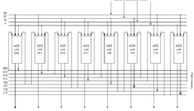
Path Metric Computation and Add-Compare-Select (ACS) Unit:

The path metric or error probability for each transition state at a particular time instant is measured as the sum of the path metric for its preceding state and the branch metric between the previous state and the present state. The initial path metric at the first time instant is infinity for all states except state 0. For each state, there are two possible predecessors. The mechanism of calculating the predecessors (and successors) the path metrics from both these predecessors is compared and the one with the smallest path metric is selected. This is the most probable transition that occurred in the original message. In addition, a single bit is also stored for each state which specifies whether the lower or upper predecessor was selected.

Figure 5: A sample implementation of a path metric unit for a specific K=4 decoder

In cases where both paths result in the same path metric to the state, either the higher or lower state may consistently be chosen as the surviving predecessor. For the purpose of this project the higher state is consistently chosen as the surviving predecessor. Finally, the state with the least accumulated path metric at the current time instant is located. This state is called the global winner and is the state from which trace back operation will begin. This method of starting the trace back operation from the global winner instead of an arbitrary state was described by Linda Bracken bury [22] in her design of an asynchronous Viterbi decoder. This greatly improves probability of finding the correct trace back path quicker and hence reduces the amount of history information that needs to be maintained. It also reduces the number of updates required to the surviving path. Both these measures result in improved energy savings. The values for the surviving predecessors (also called local winners) and the global winner are passed to Block 3.

Figure 6: A sample implementation of an ACS unit

Trace back Unit:

The global winner for the current state is received from Block 2. Its predecessor is selected in the manner. In this way, working backwards through the trellis, the path with the minimum accumulated path metric is selected. This path is known as the traceback path. A diagrammatic description will help visualize this process. The trellis diagram for a ½ K=3 (7, 5) coder with sample input taken as the received data.

Figure 7: Selected minimum error path for a ½ K=3 (7, 5) coder

(4)

minimum error path out of the two possible predecessors from that state is selected. This path is marked in blue. The actual received data is described at the bottom while the expected data written in blue along the selected path. It is observed that at time slot three there was an error in received data (11). This was corrected to (10) by the decoder.

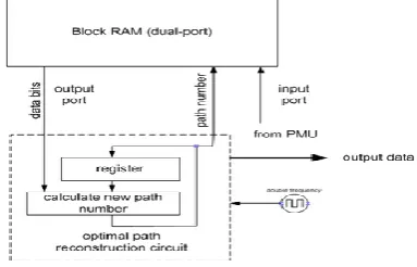
Local winner information must be stored for five times the constraint length. For a K =7 decoder, this results in storing history for 7 x 5 = 35 time slots. The state of the decoder at the time instant 35 time slots prior can then be accurately determined. This state value is passed to Block 4. At the next time slot, all the trellis values are shifted left to the previous time slot. The path metric for the last received data and compute the minimum error path is then calculated. If the global winner at this stage is not a child of the previous global winner, the traceback path has to be updated accordingly until the traceback state is a child of the previous state [22].

Figure 8: Block diagram of Trace back unit

Multiple traceback paths are possible and it may be thought that traceback up to the first bit is necessary to correctly determine the surviving path. However, it was found that all possible paths converge within a certain distance or depth of traceback [23][24]. This information is useful as it allows the setting of a certain traceback depth beyond which it is neither necessary nor advantageous to store path metric and other information. This greatly reduces memory storage requirements and hence energy consumption of the decoder. Empirical observations showed that a depth of five times the constraint length was sufficient to ensure merging of paths [8, 25]. Therefore, local winner information is stored for 35 slots (five times seven) in the decoder used for this project. Block 4. Data Input Determination Now going forwards through the traceback path, the state transitions at successive time intervals are studies and the data bit that would have caused this transition is determined. This represents the decoded output.

Determining Successors to a particular State each state is represented by 6 shift registers (in the case of a K=7 encoder or decoder). The next state can therefore be obtained by a right shift of the values of the shift registers. The first shift register is given a value of 0.

The resulting state represents the next state of the coder if the input bit was 0. By adding 32 (1x25) to this value, the next state of the coder if the input bit was 1 Determining Predecessors to a particular State In a similar way, the first predecessor can be calculated this time by a left shift of the values of the shift registers. By adding one (1x20) to this value, the value of the second predecessor to the state is derived.

Simulation Results:

RTL view of Viterbi Decoder

Timing waveform

Conclusion:

We have proposed a high speed VD design for TCM systems. The pre computation architecture that incorporates T-algorithm efficiently reducing the decoding speed appreciably. We have also analysed pre computation algorithm .where the optimal pre computation steps are calculated and discussed. This algorithm is suitable for TCM systems which always employ high rate convolution code. Finally we presented a design case. Both the ACSU and SMU are modified to correctly to decode the signal. synthesis results show that VD could improving the maximum decoding speed.

About Authors:

(5)

References:

1.Michael Purser , “Introduction to Error- correction codes”, Artech House INC,ISBN: 0-89006-784-8 ,1996 .

2.Shu Lin and Daniel J. Costello, “Error Control Coding Fundamentals And Applications”, 2nd_{edition, Prentice}

Hall, 1984.