A Review of the Extrapolation Method in Load Spectrum Compiling

(1)

0 INTRODUCTION

In engineering, many mechanical structures and components are subjected to complex and random loads, which determine the fatigue reliability and life of the machinery [1] and [2]. Thus, it is indispensable to conduct fatigue analysis and life prediction of the structures and components based on a load spectrum [3] and [4]. Currently, a load spectrum is widely used in the fields of aerospace [5] and [6], vehicle [7] and [8], wind power [9] and [10], construction machinery [11] and [12], and so on [13] and [14]. In practice, a long-term load spectrum contains the complete load information, but it is difficult to be directly measured due to the restrictions of testing technology, as well as time and cost. Therefore, it is necessary to obtain a long-term load spectrum based on a short-term one.

The traditional load spectrum compiling method multiplies a short-term load spectrum with a constant proportionality coefficient [15] to [17]. Since only the data measured in a finite time is repeated, the extreme loads that cannot be measured and have a greater impact on damage are ignored. Load extrapolation methods can overcome the above limitation of the traditional method. With the development of statistics and computer software, new methods have been applied to load extrapolation. In load spectrum

compiling, results may vary from each other with different extrapolation methods. Therefore, selecting an appropriate load extrapolation method is very important, but that is difficult in practice. For a better understanding of the methods and to provide selection guidance, several commonly used extrapolation methods are reviewed and summarized based on the literature and illustrations in this paper.

The extrapolation methods are classified as the parametric extrapolation method (PE), nonparametric extrapolation method (NPE) and quantile extrapolation method (QE). In PE, sample data is supposed to obey a known distribution, and the parameters in the function are estimated according to the load sample. In NPE, an extrapolated result is obtained because the density distribution with an arbitrary shape can be received based on a nonparametric density estimation. When the sample data has different load characteristics due to different working conditions and different operating behaviors in the testing process, QE can break the data into a series of clusters and computes the damage of each rainflow matrix. The literature and illustrations are presented to evaluate the extrapolation methods and the characteristics of various extrapolation methods, such as the critical factors, the advantages and disadvantages, and the application ranges, are summarized. Some potential research prospects are

A Review of the Extrapolation Method

in Load Spectrum Compiling

Wang, J.X. – Chen, H.B. – Li, Y. – Wu, Y.Q. – Zhang, Y.S. Jixin Wang*_{– Hongbin Chen – Yan Li – Yuqian Wu – Yingshuang Zhang}

Jilin University, School of Mechanical Science and Engineering, China

Load spectrum is the basis of fatigue analysis and life prediction in engineering, and load extrapolation is an essential procedure in determining a long-term load spectrum from a short-term one. Selecting a proper extrapolation method is of great significance when considering various forms and characteristics of load. Over the past few decades, several load extrapolation methods have been proposed, therefore the reasonability and accuracy of a load spectrum extrapolated using different methods should be of great concern. This paper conducts a literature review of commonly used extrapolation methods and proposes some future areas of research. The critical factors, the advantages and disadvantages, and the application ranges of extrapolation methods are summarized using literature and illustrations to provide guidance when selecting a method. In the future, more methods and applications of extrapolation methods will be able to be explored with the further development of statistics and computer software technology.

Keywords: short-term load spectrum, long-term load spectrum, load extrapolation, parametric extrapolation, nonparametric extrapolation, quantile extrapolation

Highlights

• This paper is focused on reviewing the commonly used extrapolation methods in load spectrum compiling in engineering; • The extrapolation methods are classified as the parametric extrapolation method, the nonparametric extrapolation method

and the quantile extrapolation method;

• Characteristics of each extrapolation method are summarized using literature and illustrations;

(2)

also discussed. The aim of this review is to be all encompassing, but this is an impossible task, so we apologize for any omissions.

1 EXTRAPOLATION METHODS

1.1 Parametric Extrapolation Method (PE)

Fitting sample data with a distribution function and estimating the parameters are included in PE. Due to the different types of sample data, PE is divided into the parameter-estimate extrapolation method (PEE) and the extreme-value extrapolation method (EVE).

1.1.1 Parameter-Estimate Extrapolation Method (PEE)

PEE is a traditional extrapolation method and extrapolates a short-term load spectrum counted from a measured load time history. PEE includes one-dimension extrapolation, in which only amplitudes accompanied by the frequencies are extrapolated, and the two-dimensional extrapolation extrapolates both the means and amplitudes together with the frequencies [18] to [20]. In practice, the two-dimensional extrapolation method is commonly used and the process is reviewed as follows:

1. Preprocess the measured load

The preprocessing mainly includes discretizing the analog signal, filtering the digital signal, eliminating the trend item, checking and eliminating the abnormal peaks [21].

2. Transform the load time history into a short- term load spectrum.

The rainflow counting method (RCM) is frequently used in PEE [16] and [18]. RCM, which was proposed by Matsuiski and Endo more than 50 years ago and developed in the following decades [22] and [23], is a procedure for determining the damaging load cycles in a load time history [24], and the cycles are usually summed into bins referenced by their mean values and amplitudes. For examples, in Wang et al. [25], the outfield load spectrum was divided into one main cycle and four sub cycles by RCM.

3. Fit the amplitudes and mean values with distribution functions.

The relationship between the mean values and frequencies usually obeys a normal distribution [20]. Meanwhile, the relationship between the amplitudes and frequencies usually obeys a Weibull distribution [26].

When the assumed variables obey a two-dimensional normal distribution, a probability density function is introduced by Holling and Mueller [27]:

f x y

e

x x y

( , )

( )

( ) ( )( )

=

− ×

− −

− ₋ − −

1

2 1 2 1

2

1

2 1 2 2

12

1 2

πσ σ ρ

ρ µ

σ ρ

µ µ σ σ ++

− 



 ( ) _

,

yµ σ2

2

22 (1)

where μ1, μ2 are the mathematical expectations of x and y, respectively, σ1, σ2 are the standard deviations of x and y, respectively, and ρ is the correlation coefficient. In the equation, μ1, μ2, σ1, σ2, ρ are all constants, and σ1 > 0, σ2 > 0, –1 < ρ < 1.

When the assumed variables obey a three-parameter Weibull distribution, the probability density function is [28] and [29]:

f x( )= x exp x ,

− −

−  

 



 − −₋



 

  

  



   −

α β ε

ε β ε

α 1 α

(2)

where x is the amplitude of the measured load, α is the shape parameter, β is the scale parameter, which equals to the value of the characteristic load, ε is the location parameter (minimum of the load). The parameters of Weibull distribution can be verified by the correlation coefficient optimization method introduced by Fu and Gao [30], and the parameter estimation methods are mainly involved in Nagode and Fajdiga [26].

4. Perform the correlation and ergodic examinations on the two functions in step 3 [20].

After these four steps, the joint probability density function is obtained. The probability 10–6_is usually chosen as the probability that the maximum load occurs [31]. The cumulative frequencies of all working conditions are calculated when the total cumulative frequency reaches 106_{. The calculation} formula to expand the frequency is [32]:

Ni'=kNi, (3)

where N_i'_{is the load cumulative frequency of the}

condition i after the extrapolation; Ni is the load cumulative frequency of the condition i before the extrapolation; k is the extending factor, k = 106_/_N_,_N_is the total load cumulative frequency before the extrapolation and can be calculated with Eq. (4) [18] and [32]:

N N

_SS _SS

f x y dx dy

m m a

a

=

'

_∫

( , )

,

1 2 1

2

(4)

(3)

Sm2 are the lower and upper limits of a load mean integration, respectively; N ′ is the load frequency

of all conditions after extrapolation; f (x, y) is the joint probability density function of the mean and amplitudes; x is the amplitude of the load; and y is the mean of the load.

5. Compile the long-term two-dimension load spectrum [20].

The process includes the amplitude classification, the mean classification, and the calculation of all cycle numbers. For convenience of the load spectrum application, it is necessary to transform the two-dimensional load spectrum into a one-two-dimensional one, which only describes the relationship between the amplitudes and frequencies. Thus, to transform the fluctuation of the mean equivalent to the amplitude, the Goodman diagram [33] is applied.

Through the above main process of PEE, the practical long-term load spectrum can be obtained. Some literature takes similar extrapolation concepts into use. In Nagode and Fajdiga [34], the scatter of a loading spectrum is extrapolated and a new process is created. Punee and Lance [35], based on the limited field data, employed statistical load extrapolation methods by estimating necessary probability distributions to predict the design loads. Nagode et al. [36] introduced two appropriate parametric models and compared them with the nonparametric methods. Agarwal and Manuel [37] extensively researched the design load spectrum of an off-store wind driven generator. With limited sample data, the obvious wave heights on wind speed were fitted by a Weibull distribution and the mean wind speed were fitted by a Rayleigh distribution, then the relevant parameters were estimated and the possible wind regimes were extrapolated.

The tail-fitting of the amplitude distribution in PEE draws little attention, which may lead to uncertainty in the fatigue analysis and life prediction based on the extrapolation results. Veers and Winterstein [10] discussed the mean, spread and tail behavior of the distribution of rainflow-range load amplitudes to approximate the distribution functions. The third moment is the skewness that provides detailed information on the tail behavior of the distribution. They improved the accuracy and reliability of the results by fitting the wind speed and turbulence intensity for various conditions, and the method provided useful information on the nature of the behavior. Moriarty et al. [38] also verified that the higher-order moment, such as the skewness

of the extreme distribution, seriously influences the extrapolated long-term loads.

1.1.2. Extreme-Value Extrapolation Method (EVE)

EVE is based on the extreme value theory (EVT) [39]. In EVE, the load spectrum made up of extreme values is extrapolated. Johannesson and Thomas [17] and Johannesson [40] divided EVE into two branches: the extrapolation in the time domain (EVET, based on the extraction methods of block maxima method and peak over threshold [41]) and in the rainflow domain (EVER, based on extraction method of level upcrossings [10]). So the process of EVE is divided into two steps: extract extreme values from a load time history and fit the extracted data.

First of all, the data extraction methods are reviewed:

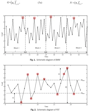
Block maxima method (BMM): It divides the continuous data X1, X2, ..., Xn, into groups according to the interval length l, and then extracts the high maxima Ml,1, Ml,2, ..., Ml,k of each group to constitute the extreme value sample. Fig. 1, which was structured according to this principle [42], shows that the key point of this method is to determine the block size reasonably [42]. This will result in a biased estimation if the block is too narrow; on the contrary, it will lead to an increase in the variance because of the lack of extreme values. Moreover, only extreme values are used in each block, which results in a low rate of data utilization, thus a large sample size is necessary.

The research on block size determination is important and the block size is usually set as one year [43] to [45].

Peak over threshold (POT): The first step is selecting the threshold level u (including umax and

umin) under certain conditions. Then the exceedances under umin and the exceedances over umax are extracted from the data, and the constitution of a new sample is made up of the exceedances. The samples of the loads

X1, X2, ..., Xn are assumed to be independent and obey the same distribution. Fig. 2, which was structured according to this principle [38] and [46], shows that

Xi will be described as the super-threshold, Yi= | Xi – u | is the exceedance, and nu as the numbers transcending the threshold, if Xi > umax or Xi < umin. By POT, the maxima above the threshold umax and the minima below the threshold umin are randomly regenerated, and only these extreme values will be extrapolated.

(4)

other hand, the level must be low enough to ensure that sufficient data will be selected to guarantee an accurate estimation of the distribution parameters, and the variance of the parameters will be decreased [47]. Johannesson [40] suggested a simple method that sets the threshold equal to the square root of the cycle number in the signal and works well in many cases [48].

Other threshold-selection methods have also been proposed, for example, Davison [49], Ledermann et al. [50] and Walshaw [51].

Level upcrossings (LU): According to Johannesson and Thomas [17], LU is proposed to obtain the maxima and minima of the load cycles, then determine the limiting shape of the rainflow matrix (RFM) and estimate the limiting RFM G[17]:

G g=

( )

_{ij i j}n =

, 1, (5a)

g E f

z

ij z

ij

= →∞

lim [ ], (5b)

where the elements fij of Fz are the number of rainflow cycles in distance z, with a minimum in class i and a maximum in class j. Fz is the rainflow matrix in distance z.

This approach is based on an asymptotic theory for the crossings of extreme (high and low) levels. First, obtain a measured RFM F[17]:

F=

( )

f_{ij i j}n ₌

, 1, (6)

where fij is the number of the cycle with minimum i and maximum j.

Then, calculate the LU from F and determine a suitable threshold. The level upcrossings spectrum is calculated as follows [17]:

N₌

_{( )}

n_{k k}n

=1, (7)

0 5 10 15 20 25 30 35 40 45 50

0 1 2 3 4 5 6

Time

Lo

ad

l l

l

Block 2

l Block 3

Block 1 Block 4

Fig. 1. Schematic diagram of BMM

0 5 10 15 20 25

0 1 2 3 4 5 6 7 8 9

Time

Lo

ad

u

u max

min

X

i

Y

i

Y

i

(5)

where nk is the accumulative cycle number from the load level i below k to the load level j above k:

nk fij

i k j

= < <

∑

.

After reviewing the extraction methods, the fitting process will be described.

In the time domain, POT is more frequently used, and taking it as an example in this section: the load threshold is u and the load exceedances above or below u usually obey the Generalized Pareto distribution (GPD), introduced by Pickands [52], Cerrini et al. [53] and Lourenco [54]. The cumulative distribution function for GPD is [53]:

F x

( )

 −k x u− k 

  =1- 1

1

α( ) ,

/

(8)

where u is the predetermined threshold, x is the measured load, x – u is the exceedance, k is the shape parameter, and α is the scale parameter.

When k = 0, the GPD turns into an exponential distribution [53]:

F x

( )

− −m 

 

  =1 exp

α , (9)

where m = | x – u | is the ‘mean exceedance’.

When the exceedances obey the exponential distribution, the estimated parameter is the mean of the exceedances [53]:

m

N Zi

i N

= =

∑

1

, (10)

where Zi is the exceedance, N is the number of exceedances.

The parameter estimations for the GPD have been discussed by Davison [49], Hosking and Wallis [55], as well as Smith [56].

In the rainflow domain, the shape of the level upcrossing intensity above the threshold is estimated. The level upcrossing obeys GPD and the estimates of the parameters in GPD are calculated using relative estimation techniques [17]. Then, an estimate of the cumulative RFM is calculated as [17]:

n n n

n n

ij i j

i j

=

+ , (11)

Thus, the corresponding estimation of the RFM

Frfc_is_[17]_:

Frfc f

ij i j n

=

( )

₌

, 1, (12)

where fij is the cumulative frequency number from the load level i to the load level j,

fij = ni+1,j–1– ni,j–1 – ni+1,j + ni,j .

The main process of EVE has been sketched out and the practical operation is conducted based on the technical software package, for example, WAFO [57]. Johannesson [40] conducted the 100-fold extrapolation and compared the extrapolated load spectrum with the 100 repetitions of the measured load spectrum, then it was found that the extrapolation result was more reasonable because it agreed well with the observed load spectrum. Due to the uncertainty of wind conditions, the extreme load on a wind turbine is usually difficult to determine. In 2008, Collani et al. [58] put forward a reliable method named LEXPOL [59] to solve the problem. For the sake of different environments, Agarwal and Manuel [60] deduced the long-term loads with POT and a three-parameter Weibull distribution, then a good extrapolated result was obtained. A quadratic distortion of the Gumbel distribution was introduced by Natarajan et al. [61] and Natarajan and Holley [62] and it was used to fit the tail of the extreme loads on a wind turbine. Based on this method, the finite sample data was extrapolated to 50 years. In addition, an extrapolation method based on the mean and standard deviation of extreme values was proposed by Moriarty [63], where subjectivity of the parametric extrapolation was avoided.

1.2 Nonparametric Extrapolation Method (NPE)

NPE, which was proposed by Dressler et al. in 1996 [64], uses a nonparametric statistical approach to get the statistical probability distribution. In NPE, the nonparametric density estimation reduces the subjectivity of empirical hypothesis because it makes no assumptions on the distribution of the sample data. As a result, the extrapolated load spectrum is not influenced by the characteristics of the sample data.

The kernel estimation can be employed for nonparametric density estimation [65] and [66]. The estimation transforms a discrete histogram of sample data into a probability distribution.

Suppose X1, X2, ..., Xn are observed samples from a common distribution with density f (·). The kernel density estimation (KDE) of f (·) is [64]:

f x

nh K x Xh

h i

i n

 _{( )}₌ ₍ − _),

=

∑

1

(13)

where K is the kernel function and h is the bandwidth. To assure the reasonability of the KDE function f xh

 _{( )}_{, kernel}_K_satisfies_[64]_:

K x

( )

≥

,

K x dx

( )

=

,

−∞ +∞

∫

0

1

(14)

(6)

1. Transform the measured load time history into a rainflow counted histogram.

2. Select the appropriate kernel function and bandwidth, then use the nonparametric method in combination with the Monte Carlo method [67] to extrapolate the RFM that is obtained from the lifecycle one.

3. Reconstruct a new load spectrum from the RFM lifecycle.

For NPE, a lot of research was conducted on the selection of the kernel function and bandwidth. Wang et al. [68] proposed a selection method for the kernel function and the multi-criteria decision making technique was successfully used to solve the problem of the kernel function selection. For the bandwidth selection, Heidenreich et al. [69] reviewed the bandwidth selections for the kernel density estimation and some of the methods can be used in NPE. Sheather [70] proposed two kinds of bandwidth determination methods: Sheather-Jones plug-in bandwidth and least squares cross validation. The Sheather-Jones plug-in bandwidth was widely used because of its overall good performance, but this method was prone to be over-smoothing in some situations. As a supplement, it was solved by the least squares cross validation. Besides, Bayesian methods [71] and [72] were used to estimate the adaptive bandwidth and adaptive bandwidth matrix in univariate and multivariate KDEs.

For the applications of NPE, Dressler et al. [64] transformed the discrete rainflow matrix into a smooth function that is more accessible with a kernel density estimator. In the literature, the RFM is seen as two-dimensional histograms of the opening and closing points of hystereses, and can only be described by a nonparametric method due to its arbitrary shapes. Socie [73] employed nonparametric kernel smoothing techniques to transform the discrete rainflow histogram of cycles into a probability density histogram and extrapolated the short-term measured load to an expectedly long-term one. The key role of the bandwidth in KDE is also indicated in the literature. Johannesson [17] considered that kernel smoothing is a feasible smoothing technique and well-established statistical method for nonparametric estimation. A kernel smoother method is also proposed to estimate the RFM for the cycles with small and moderate amplitudes. Mattetti et al. [74] extrapolated the RFM by NPE in carrying out of accelerated structural tests of tractors.

1.3 Quantile Extrapolation Method (QE)

Considering the influences of different working conditions and operating behaviours in engineering, load extrapolation is difficult. Under these circumstances, the quantile extrapolation method (QE) is capable of taking various conditions and behaviors into consideration and optimizing the extrapolation results.

The main process of QE is as follows [64]:

1. Break the data set of the rainflow-counted histogram into a series of clusters B1, B2, ..., Bm with similar variables and damages.

2. Compute the damage of each original RFM R by Miner’s rule. Damage vectors [64]:

(

( ), ..., ( ))

( ), ..., ( )) D R

D R

m

n m n

1 1 1

1 

are obtained for all original RFMs, where

R1, R2, ..., Rn represent the influence of various conditions and behaviors.

3. Estimate the expected damage for the x% quantile. The quantile damage vector (q1,q2,..., qm), which describes the damage distribution between the individual clusters of the rainflow matrix, is used to construct the rainflow matrix. The original rainflow matrix is superposed such that [64]:

RG =R1+ ⋅⋅⋅ +Rn. (15)

4. Construct and extrapolate the corresponding RFM into a matrix, the extrapolation of the resulting matrix [64] is:

R_E=extrapol R( _G), (16)

(7)

In load spectrum compiling, QE is usually combined with other extrapolation methods and it is also an important component in computer software.

1.4 Classification of the Extrapolation Methods

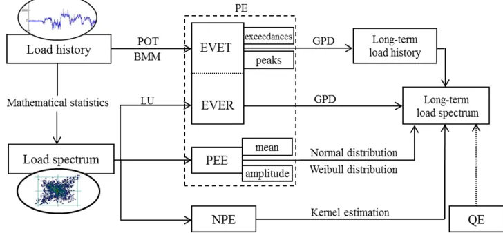
The extrapolation methods are integrated into one figure for clarity. As shown in Fig. 3, the classifications and pivotal elements of the methods are reflected.

2 CASE ANALYSIS

In this section, some illustrations and examples are displayed to evaluate and demonstrate the extrapolation methods.

2.1 Case Analysis of PEE

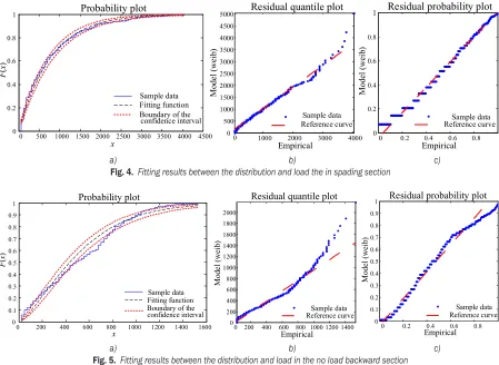
In PEE, distributions of the sample data affect the extrapolation results [26]. In this section, the load on an axle shaft of a loader powertrain was taken as the research object. According to the obvious segment working characteristics of a loader, the operation process was divided into six sections. In this paper, the load on the axle shaft in the spading and the no load backward sections were illustrated to verify the characteristics of PEE. Amplitudes of the load with different characteristics and distributions were focused on. The Weibull distribution was employed, with the fitting results shown in Fig. 4 and Fig. 5. Compared with Fig. 4a, the fitting in middle of Fig. 5a diverges from the distribution function more remarkably. In Fig. 5b, the tail of the fitting seriously diverges from the skew line, as in Fig. 5c. Based on the comparison, the conclusion is that the fitting between the function

and load in the spading section is better. So, when PEE is applied to extrapolating the load on an axle shaft with different characteristics, the repeatability of the result will be influenced. Therefore, the distributions of the sample data will influence the fitting error in PEE, and the fitting error will lead to an inaccuracy in the extrapolation results.

2.2 Case Analysis of EVE

In EVE, both the data extracting and fitting function selection will affect the extrapolation results. During the data extracting process, selection of the threshold or block size is important [75] to [78], as this will influence the data utilization ratio and the distribution characteristics of the extreme values. Fitting precisions vary from each other due to different load characteristics, thus the extrapolation results of EVE are dependent on the fitting precisions. Several examples will illustrate the influences of different thresholds on the fitting precisions.

In this section, the load on an axle shaft of a loader powertrain in the spading section was used. The automatic threshold selection method, which was proposed in Thompson [79], was adopted to determine the original threshold. In data processing, based on the sample data, 2897.3 Nm was set as the automatic threshold and the number of extreme values was 5734, thus 5734 exceedances were calculated. With GPD, the exceedances were fitted with the parameters estimated by the maximum likelihood method, and the results are shown in Fig. 6.

In order to reflect the effects of thresholds on fitting precisions, 2000 Nm and 3500 Nm were selected as the other thresholds to extract values, thus

(8)

the values were fitted with the same distribution and parameter estimation method. The fitting results are shown in Fig. 7 and Fig. 8. Compared with Fig. 6, the deviations between the data points (the extreme values) and the fitting distribution in Fig. 7 and Fig. 8 are obvious, especially in plot a and b of the figures. So, with different thresholds, the fitting precisions are different, which will influence the results from EVE. On the basis of the comparison, the significance of selecting the threshold or block size is verified.

The influence of the distribution function on the extrapolation results also needs to be considered. In Johannesson [17], GPD was used to extrapolate the simulated Markov load with the maximum likelihood estimation and the result was shown in Fig. 9a [17]. Thus, the exponential distribution was adopted to extrapolate the same load, the result was shown in Fig. 9b [17]. Making a comparison between the two parts in Fig. 9, the exponential tail in Fig 9b yields a straight line in the log-scale that tends to overestimate the intensity for extreme crossings [17]. Therefore, the conclusion can be drawn that GPD gives a better extrapolation and thus verifies the importance of selecting a suitable distribution function.

There are two branches in EVE: EVET and EVER. Making a comparison of the two branches, it is easy to find some distinctions, such as the application domains, the fitting functions and the types of the extrapolation results.

In Johannesson [40], EVET and EVER were both applied to extrapolate the load of a train and a car, respectively, and the results are show in Fig. 10.

Fig. 10 allows some comparisons between EVET and EVER to be noted [40]:

1. EVET generates the extrapolated load cycle directly based on the measured load time history, so the outcome is more reliable;

2. EVET is more robust because it is only on the basis of EVT, while the EVER uses an additional extreme value approximation for the shape of the rainflow matrix;

3. The limitation in the extrapolation multiple of EVET is that the extrapolated result is an N-fold extrapolated load. In EVER, the extrapolated result is a limited rainflow matrix, which represents infinite repetitions.

4. Results extrapolated by EVET are usually adopted into a fatigue test or as the input load 0 500 1000 1500 2000 2500 3000 3500 4000 4500

0 0.2 0.4 0.6 0.8 1 x F ( x ) Probability plot

0 0.2 0.4 0.6 0.8 1

0 0.2 0.4 0.6 0.8 1 Empirical M od el (we ib )

Residual probability plot

Sample data Fitting function Boundary of the

confidence interval _{Reference curve}Sample data

1000 2000 3000 4000

500 1000 1500 2000 2500 3000 3500 4000 4500 5000 Empirical M od el (we ib )

Residual quantile plot

Sample data Reference curve

0 0

a) b) c) Fig. 4. Fitting results between the distribution and load the in spading section

200 400 600 800 1000 1200 1400 200 400 600 800 1000 1200 1400 1600 1800 2000 Empirical M od el (we ib )

0 0.2 0.4 0.6 0.8 1 0 0.1 0.2 0.3 0.4 0.5 0.6 0.7 0.8 0.9 1 Empirical M od el (we ib )

Sample data

Reference curve Reference curveSample data

0 200 400 600 800 1000 1200 1400 1600 0 0.1 0.2 0.3 0.4 0.5 0.6 0.7 0.8 0.9 1 x F ( x ) Probability plot Sample data Fitting function Boundary of the confidence interval

0 0

(9)

for life prediction. However, if the target is to extrapolate a load spectrum and acquire the relationship between the load and frequencies over the whole life, EVER will be an appropriate selection because it has high efficiency and it can estimate the shape of the load spectrum for an infinitely long measurement. Sometimes, the extrapolation results can be transformed. Load in

the time domain can be transformed into rainflow

domain by RCM. The Markov method [80]

can also be used to transform the load from the rainflow domain to the time domain. However, the accuracy of the results will be influenced during the transforming process.

0 200 400 600 800 1000 1200 1400

200 400 600 800 1000 1200 200 400 600 800 1000 1200 Empirical M od el (g en pa r)

0 0.2 0.4 0.6 0.8 1

0 0.2 0.4 0.6 0.8 1 Empirical M od el (g en pa r)

Sample data

Reference curve Reference curveSample data Sample data

Fitting distribution Boundary of the confidence interval

0 0

a) b) c) Fig. 6. Threshold u = 2897.3, fitting results

0 500 1000 1500 2000 2500

500 1000 1500 2000 0 500 1000 1500 2000 Empirical M od el (g en pa r)

0 0.2 0.4 0.6 0.8 1 0 0.2 0.4 0.6 0.8 1 Empirical M od el (g en pa r)

Sample data

Reference curve Sample dataReference curve Sample data

Fitting function Boundary of the confidence interval

0

a) b) c) Fig. 7. Threshold u = 2000, fitting results

0 100 200 300 400 500 600 700

100 200 300 400 500 600 0 100 200 300 400 500 600 Empirical M od el (g en pa r)

0 0.2 0.4 0.6 0.8 1

0 0.2 0.4 0.6 0.8 1 Empirical M od el (g en pa r)

Sample data

Reference curve Sample dataReference curve Sample data

Fitting function Boundary of the confidence interval

0

(10)

69

A Review of the Extrapolation Method in Load Spectrum Compiling

2.3 Case Analysis of NPE

In NPE, kernel estimation provides a convenient way to estimate the probability density [65] and [81]. In kernel estimation, both kernel function [68] and bandwidth [66] are of great concern.

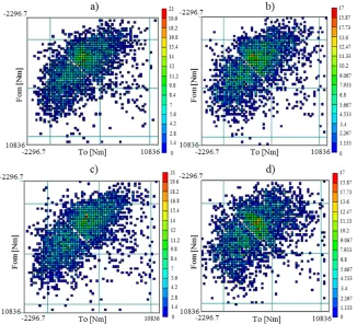
In Wang et al. [68], the selection of the kernel function was considered. Four kinds of kernel functions were illustrated; the extrapolation results are shown in Fig. 11 using these kernel functions. [68]. As shown in Fig. 11, the results based on different kernel functions vary from each other, especially the extrapolated extreme loads.

When NPE was first proposed by Dressler et al. in 1996 [64], the importance of bandwidth was emphasized and this was also confirmed in the following research [64], [66] and [82]. Compared with the kernel function, extrapolation results are more sensitive to the bandwidth [64] and [66]. So far, only two kinds of bandwidths are commonly applied to data extrapolation. They are the fixed and the adaptive bandwidth [64] and [66]. In this section,

in order to verify the influence of the bandwidths on the probability density, a fixed bandwidth with different values will be discussed. As shown in Fig. 12, the solid line represents the probability density based on the automatic fixed bandwidth hs = 0.5187, where the other two lines represent the densities with the bandwidths hs = 0.2 and hs = 1 respectively. As shown in Fig. 12, when the bandwidth equals 0.2, the double-peak occurred at the peak of the density and the fluctuation in the second half was obvious. When the bandwidth increases to 1, the maximum density declined to a large extent. So, with different bandwidths, the probability density, which is directly related to the extrapolation result, makes a big difference.

2.4 Case Analysis of QE

Based on the former discussion on QE, the principle in Dressler et al. [64] is important and comprehensive. In Dressler et al. [64], based on four figures (Figs. 10 to 13 in K. Dressler et al. [64]), the importance and

a) b)

Fig. 9. Extrapolation of level upcrossing intensity; a) with GPD; b) with EXP E X T R A P O L AT I O N O F L OA D H I S TO R I E S A N D S P E C T R A[17] 207

1000 101 102 103 104 105 106 107 5 10 15 20 25 30 35

Cumulative number of cycles

Amplitude / MPa

(a) Load spectrum – Train

Time extrapolation Rainflow extrapolation Measurement

1000 101 102 103 104 105 106 1 2 3 4 5 6 7 8

Amplitude / kN

(b) Load spectrum – Car

Fig. 8Hundred-fold extrapolations comparing time and rainflow domain methods.

Another advantage of the time domain method could be that the generated sequence of cycles is more realistic since it is directly based on a measured sequence.

If our goal is to extrapolate the load spectrum, the method of rainflow extrapolation has the properties of being more computationally efficient, and estimates the shape of the load spectrum for an infinitely long

measure-ment. However, the time domain method is more robust, since it only uses the extreme value theory for extrapo-lating to extreme load levels, while the rainflow domain method uses an additional extreme value approximation for the shape of the rainflow matrix.

Acknowledgements

The author thanks Bombardier Transportation and PSA Peugeot Citro¨en for their support, and for permission to use their load data in the examples. Further the author is thankful to Professor Jacques de Mar´e and Dr Thomas Svensson for valuable comments and discussion.

R E F E R E N C E S

1 Davison, A. C. and Smith, R. L. (1990) Models for exceedances over high thresholds.J. Royal Stat. Soc., Ser. B52, 393–442. 2 Castillo, E. (1988)Extreme Value Theory in Engineering.

Academic Press, San Diego.

3 Coles, S. (2001)An Introduction to Statistical Modelling of Extreme Values. Springer Verlag, London.

4 Dressler, K., Gr ¨under, B., Hack, M. and K ¨ottgen, V. B. (1996) Extrapolation of rainflow matrices.SAE Technical Paper960569. 5 Grimshaw, S. D. (1993) Computing maximum likelihood

estimates of the generalized Pareto distribution.Technometrics 35, 185–191.

6 Grubisic, V. (1994) Determination of load spectra for design and testing.Int. J. Veh. Des.15, 8–26.

7 Hosking, J. R. M. and Wallis, J. R. (1989) Parameter and quantile estimation of the generalized Pareto distribution.

Technometrics29, 339–349.

8 Johannesson, P. and Thomas, J.-J. (2001) Extrapolation of rainflow matrices.Extremes4, 241–262.

9 Leadbetter, M. R., Lindgren, G. and Rootz´en, H. (1983)

Extremes and Related Properties of Random Sequences and Series. Springer Verlag, New York.

10 Rychlik, I. (1996) Simulation of load sequences from rainflow matrices: Markov method.Int. J. Fatigue18, 429–438. 11 Socie, D. (2001) Modelling expected service usage from

short-term loading measurements.Int. J. Mater. Prod. Technol. 16, 295–303.

12 Thomas, J.-J., Perroud, G., Biognonnet, A. and Monnet, D. (1999) Fatigue design and reliability in the automotive industry. In:Fatigue Design and Reliability, ESIS publication 23(Edited by G. Marquis and J. Solin). Elsevier, pp. 1–12.

E X T R A P O L AT I O N O F L OA D H I S TO R I E S A N D S P E C T R A 207

100 101 102 103 104 105 106 107 0 5 10 15 20 25 30 35

Amplitude / MPa

(a) Load spectrum – Train

100 101 102 103 104 105 106 0 1 2 3 4 5 6 7 8

Amplitude / kN

(b) Load spectrum – Car

Fig. 8Hundred-fold extrapolations comparing time and rainflow domain methods.

Another advantage of the time domain method could be that the generated sequence of cycles is more realistic since it is directly based on a measured sequence.

If our goal is to extrapolate the load spectrum, the method of rainflow extrapolation has the properties of being more computationally efficient, and estimates the shape of the load spectrum for an infinitely long

measure-ment. However, the time domain method is more robust, since it only uses the extreme value theory for extrapo-lating to extreme load levels, while the rainflow domain method uses an additional extreme value approximation for the shape of the rainflow matrix.

Acknowledgements

The author thanks Bombardier Transportation and PSA Peugeot Citro¨en for their support, and for permission to use their load data in the examples. Further the author is thankful to Professor Jacques de Mar´e and Dr Thomas Svensson for valuable comments and discussion.

R E F E R E N C E S

1 Davison, A. C. and Smith, R. L. (1990) Models for exceedances over high thresholds.J. Royal Stat. Soc., Ser. B52, 393–442. 2 Castillo, E. (1988)Extreme Value Theory in Engineering.

Academic Press, San Diego.

3 Coles, S. (2001)An Introduction to Statistical Modelling of Extreme Values. Springer Verlag, London.

4 Dressler, K., Gr ¨under, B., Hack, M. and K ¨ottgen, V. B. (1996) Extrapolation of rainflow matrices.SAE Technical Paper960569. 5 Grimshaw, S. D. (1993) Computing maximum likelihood

estimates of the generalized Pareto distribution.Technometrics 35, 185–191.

6 Grubisic, V. (1994) Determination of load spectra for design and testing.Int. J. Veh. Des.15, 8–26.

7 Hosking, J. R. M. and Wallis, J. R. (1989) Parameter and quantile estimation of the generalized Pareto distribution.

Technometrics29, 339–349.

8 Johannesson, P. and Thomas, J.-J. (2001) Extrapolation of rainflow matrices.Extremes4, 241–262.

9 Leadbetter, M. R., Lindgren, G. and Rootz´en, H. (1983)

Extremes and Related Properties of Random Sequences and Series. Springer Verlag, New York.

10 Rychlik, I. (1996) Simulation of load sequences from rainflow matrices: Markov method.Int. J. Fatigue18, 429–438. 11 Socie, D. (2001) Modelling expected service usage from

short-term loading measurements.Int. J. Mater. Prod. Technol. 16, 295–303.

12 Thomas, J.-J., Perroud, G., Biognonnet, A. and Monnet, D. (1999) Fatigue design and reliability in the automotive industry. In:Fatigue Design and Reliability, ESIS publication 23(Edited by G. Marquis and J. Solin). Elsevier, pp. 1–12.

c

2006 The Author. Journal compilationc2006 Blackwell Publishing Ltd.Fatigue Fract Engng Mater Struct29, 201–207 a) b)

(11)

necessity of QE were confirmed, and determinations of the clusters were shown.

The choice of the solution parameters in QE was also emphasized in Dressler et al. [64]. On one hand, the extrapolation results are highly dependent on the determination of the clusters B1, B2, ..., Bm , which can

be adjusted according to different conditions or be defined invariant of the data analyzed. On the other hand, it is important to test the resultant vectors for Gaussian distribution and the determination of the x% matrix will be much easier with the vectors.

Fig. 11. Comparison among extrapolated results based on different kernel functions; a) circular; b) mean-basedellipse; c) range-based ellipse; d) epanechekov

(12)

3 SUMMARIES OF THE EXTRAPOLATION METHODS

Characteristics of the extrapolation methods are summarized from three aspects (the critical factors, the advantages and disadvantages, and the application ranges of each extrapolation method) based on the previous sections.

3.1 Critical Factors

Critical factors in each extrapolation method are summarized in Table 1. These factors are mentioned and emphasized in the preceding part based on the literature and illustrations.

3.2 Advantages and Disadvantages

Based on the literature and illustrations, the advantages and disadvantages of each extrapolation method are summarized in Table 2.

3.3 Application Ranges

Different extrapolation methods have their own application ranges. In practice, the application ranges of a certain extrapolation method are not categorical. A method has to be selected on the basis of the practical situation. Application ranges of the methods in this paper are mainly based on the load characteristics and extrapolation purposes, which are summarized as follows.

PEE: For sample data, when the stationary test for a certain distribution is qualified, PEE will be an appropriate selection. However, when convenience and efficiency of data processing is required instead of the accuracy, PEE can be considered. For example, in Xiang [20], the distributions of the load amplitudes and mean values fit well with the fitting functions and they are independent, so PEE is adopted.

EVE: EVE is a proper choice in circumstances where the sample data is composed of extreme load. For example, the data in the fields of wind speed and engineering machinery could be extrapolated by EVE. Furthermore, if the purpose is to produce a load time history for fatigue test and fatigue life evaluation, EVET is a better choice because it is capable of extrapolating the load time history directly. EVER is more applicable for accurate load spectrum extrapolation of large load cycles. EVER is also an appropriate choice in circumstances where the load spectrum can be modeled as a Gaussian or Markov model.

NPE: NPE is limited by the sample size of large load cycles. If the sample size is enough, NPE may be a better choice. For extrapolating medium and small load cycles, NPE can be used. When it is difficult to

Table 2. Advantages and disadvantages of each extrapolation method

Extrapolation

method Advantages Disadvantages

PEE • • Computes efficiently Considers the influences of both mean value and [20] and [7]; amplitude of the sample data [19] and [20].

• Relies on the distribution of the measured data; • There is subjectivity in selecting a parameter-estimate

method [26].

EVET

• Gets a load time history directly; • Generated sequence of cycles is realistic; • Robust;

• Considers the influence of extreme values.

• The block size and threshold selection has a great influence on the extrapolation accuracy.

• Relies on distributions of the sample data ;

EVER

• Estimates the shape of the load spectrum for an infinitely long measurement;

• Available for large cycles.

• Produces a rainflow matrix and needs to be converted into a time signal;

• Choice of the threshold is difficult. • Relies on distributions of the sample data;

NPE • • Independent of the distributions of the sample data Effective estimation of the load spectrum with arbitrary [64]; shapes [64].

• Large amount of sample data is needed [64] and [66]; • The kernel function and bandwidth selection is influential.

QE • The extrapolated samples consider the influence of _{different conditions and operating behaviours.} • Influential step is breaking the sample data into a series of _clusters_[64]_.

Table 1. Critical factors in each extrapolation method

Extrapolation

method Critical factor

PEE Distribution prediction of the sample dataSelection of the distribution function Parameter estimation

EVE

Threshold or block size determination Distribution prediction of the sample data Selection of the distribution function Parameter estimation

NPE Selection of the kernel function Bandwidth determination

(13)

define the model of the distribution accurately or there is little dependence on the distribution of the sample data, NPE may be a good choice. For example, in the field of vehicles, the load may be extrapolated by NPE [68].

QE: When different working conditions and operating behaviors are considered, QE will be useful in data processing. For example, due to the complex working conditions of engineering machinery, the load in the field may be extrapolated with QE [4].

4 DISCUSSIONS

Due to the limited paper length, there are some deficiencies in this review. For example, in PE, some other distribution functions should be reviewed, such as the logarithmic normal distribution in PEE and the Rayleigh distribution in EVE. In EVE, the importance of the threshold or block size is verified, but the selecting methods of the threshold or block size should be further discussed. In NPE, the influence of bandwidths on the density distribution is verified, but the difference between the adaptive and fixed bandwidth requires further comparison, and which one is better for a certain situation is not concluded. For QE, where different working conditions are concerned, the process and details of combining QE with other methods are not fully reviewed. Furthermore, one purpose of this review is to provide guidance on selecting an appropriate load extrapolation method for a certain case. In this review, only part of the guidance is involved, so further research on completing the guidance may be useful.

5 CONCLUSIONS

Load extrapolation provides a feasible and reliable approach to obtaining a long-term load spectrum for fatigue analysis and life prediction in engineering. Several commonly used extrapolation methods are reviewed in this paper. Some conclusions are as follows:

1. PEE and EVE are both included in PE. PEE is based on the distributions of the sample data. Specific distribution functions are employed to fit and the parameters in the functions are estimated according to the sample data. The PEE process is simple and efficient, but some errors may arise in the results;

2. EVE is based on EVT. Extreme values obtained by extraction methods such as BMM, POT, and LU are extrapolated by a process similar to PEE, but the distribution functions are usually different.

EVE is valid for the load time history with large load cycles, but selecting a proper threshold or block size usually requires further consideration; 3. For extrapolating small and moderate loads, NPE

can be applied accompanied by kernel estimation. There is no need to predict the distributions of the sample data and estimate the parameters of the functions in NPE. The rationality of the results extrapolated by NPE is directly influenced by the kernel function and bandwidth, especially the latter;

4. The extrapolation methods mentioned above could be combined with QE when the influences of different working conditions and operating behavior are considered. In QE, determining the solution parameters is an important step.

Some potential future research directions are also predicted:

First, a difference between the extrapolated and measured load always exists, thus an evaluation criterion should be set to evaluate the difference, which may provide important guidance for selecting the appropriate method. Second, the references and applications are mainly about the field of engineering in this review. In fact, extrapolation is being used in many other fields, such as weather prognosis, hydrological forecasting, and financial analysis. Methods from other fields can be borrowed and adopted in another field. In addition, limited by the physical circumstances in engineering, many load spectra have maximum or minimum limits. Extrapolating the sample data appropriately within these limits is challenging. Therefore, research on the appropriate extrapolation may provide another way to optimize the results.

6 ACKNOWLEDGEMENTS

This work was supported by National Natural Science Foundation of China (No. 51375202 and 51075179).

7 REFERENCES

[1] Rychlik, I. (1996). Fatigue and stochastic loads. Scandinavian

Journal of Statistics, vol. 23, no. 4, p. 387-404.

[2] Maisch, M., Bertsche, B., Hettich, R. (2006). An approach

to online reliability evaluation and prediction of mechanical

transmission components. International Journal of Automation

and Computing, vol. 3, no. 2, p. 207-214, DOI:10.1007/ s11633-006-0207-5.

[3] Bandemer, H. (1980). Statistical analysis of reliability and

(14)

Mathematics and Mechanics, vol. 60, no. 10, p. 544,

DOI:10.1002/zamm.19800601021.

[4] Zhang, Y.S. (2014). Research on the Load Spectra Acquisition

and Application of Loader Powertrain, PhD Thesis, Jilin University, Changchun. (in Chinese)

[5] Owczarek, W., Rodzewicz, M. (2009). Investigations into glider

chassis load spectrum. Fatigue of Aircraft Structures, no. 1, p.

150-169, DOI:10.2478/v10164-010-0014-x.

[6] Katcher, M. (1973). Crack growth retardation under aircraft

spectrum loads. Engineering Fracture Mechanics, vol. 5, no.

4, p. 793-818, DOI:10.1016/0013-7944(73)90052-0.

[7] Rui, Q., Wang, H.Y. (2011). Frequency domain fatigue

assessment of vehicle component under random load

spectrum. Journal of Physics: Conference Series, vol. 305, no.

1, p. 1-9, DOI:10.1088/1742-6596/305/1/012060.

[8] Zhang, L.P., Guo, L.X. (2011). The vehicle dynamic load

identification under the excitation of random road surface. Advanced Materials Research, vol. 299-300, p. 255-259,

DOI:10.4028/www.scientific.net/amr.299-300.255.

[9] Moriarty, P.J., Holley, W.E., Butterfield, S. (2002). Effect of

turbulence variation on extreme loads prediction for wind

turbines. Journal of Solar Energy Engineering, vol. 124, no. 4,

p. 387–395, DOI:10.1115/1.1510137.

[10] Veers, P.S., Winterstein, S.R. (1998). Application of measured

load to wind turbine fatigue and reliability analysis. Journal

of Solar Energy Engineering, vol. 120, no. 4, p. 233-239,

DOI:10.1115/1.2888125.

[11] Wang, J.X., Liang, Y.L., Wang, Z.Y., Wang, N.X., Yao, M.Y., Sun, Y.F. (2011). Test and compilation of load spectrum of

hydraulic cylinder for earth moving machinery. Advanced

Science Letters, vol. 4, no. 6-7, p. 2022-2026, DOI:10.1166/ asl.2011.1661.

[12] Wang, J., Hu, J., Wang, N., Yao, M., Wang, Z. (2012). Multi-criteria decision-making method-based approach to determine

a proper level for extrapolation of Rainflow matrix. Proceedings

of the Institution of Mechanical Engineers, Part C: Journal of Mechanical Engineering Science, vol. 226, no. 5, p.

1148-1161, DOI:10.1177/0954406211420212.

[13] Yamada, K., Cao, Q., Okado, N. (2000). Fatigue crack growth

measurements under spectrum loading. Engineering Fracture

Mechanics, vol. 66, no. 5, p. 483-497, DOI:10.1016/S0013-7944(99)00143-5.

[14] O’Connor, A., Caprani, C., Belay, A., (2002). Site-specific probabilistic load modeling for bridge reliability analysis. Assessment of Bridges and Highway Infrastructure, p. 97-104.

[15] Heuler, P., Klatschke, H., (2005). Generation and use of standardized load spectra and load–time histories. International Journal of Fatigue, vol. 27, no. 8, p. 974-990,

DOI:10.1016/j.ijfatigue.2004.09.012.

[16] Johannesson, P., Speckert, M. (eds.) (2013). Guide to Load Analysis for Durability in Vehicle Engineering. John Wiley &

Sons Ltd, Chichester, DOI:10.1002/9781118700518.

[17] Johannesson, P., Thomas, J.J., (2001). Extrapolation of

rainflow matrices. Extremes, vol. 4, no. 3, p. 241-262,

DOI:10.1023/A:1015277305308.

[18] Chen, A.Y., Gao, Z.T. (1986). Statistical treatment of

two-dimensional random fatigue loads and its application. Journal

of Beijing Institute of Aeronautics and Astronautics, no. 1,

p. 75-85, DOI:10.13700/j.bh.1001-5965.1986.01.009. (in

Chinese)

[19] Ling, J., Gao, Z. T., (1992). The statistical treatment for fatigue loads of a mechanical structure under multi-operating

conditions. Journal of Mechanical Strength, vol. 14, no. 2, p.

31-34. (in Chinese)

[20] Xiang, C.L. (2007). Dynamics of Armored Vehicle Transmission System, National Defense Industry Press, Beijing.

[21] Jia, H.B. (2009). Study on the Test and Generation Methods about Load Spectrum of Wheel Loader Driveline. Jilin University, Changchun.

[22] Downing, S.D., Socie, D.F. (1982). Simple rainflow counting

algorithms. International Journal of Fatigue, vol. 4, no. 1, p.

31-40, DOI:10.1016/0142-1123(82)90018-4.

[23] Hong, N. (1991). A modified rainflow counting method. International Journal of Fatigue, vol. 13, no. 6, p. 465-469,

DOI:10.1016/0142-1123(91)90481-d.

[24] Rice, R.E. (1988). Fatigue Design Handbook, 2nd_edition_,

AE-10, Society of Automotive Engineers.

[25] Wang, R.Q., Wei, J.M. Hu, D.Y., Shen, X.L, Fan, J, (2013). Investigation on experimental load spectrum for high and low

cycle combined fatigue test. Propulsion and Power Research,

vol. 2, no. 4, p. 235-242, DOI:10.1016/j.jppr.2013.11.004.

[26] Nagode, M., Fajdiga, M. (1998). A general multi-modal probability density function suitable for the rainflow ranges

of stationary random processes. International Journal of

Fatigue, vol. 20, no. 3, p. 211-223, DOI:10.1016/s0142-1123(97)00106-0.

[27] Holling, D., Mueller, A. (1973). Accelerated fatigue-testing

improvements from road to laboratory. SAE Automobile

Engineering Meeting, vol. 2, p. 730564, DOI:10.4271/730564.

[28] Weibull, W., (1961). Fatigue Testing and Analysis of Results. Macmillan Company, New York.

[29] Bethea, R.M., Rhinehart, R.R. (1991). Applied Engineering Statistics. Marcel Dekker, New York.

[30] Fu, H.M., Gao, Z.T. (1990). An optimization method of coefficient optimization for determining a three-parameter

Weibull distribution. Acta Aeronautica et Astronautica Sinica,

vol. 11, no. 7, p. 323-327. (in Chinese)

[31] IEC 61400-1 (2005). Wind turbines-Part 1: Design requirements. 3rd_edition_{. International Electrotechnical}

Commission, Geneva

[32] Liu, Y., Zhang X. F., Wang Z.Y., Liu Q.S., Wang J.X. (2011).

Contrast of extrapolations in compiling load spectrum. Modern

Manufacturing Engineering, no. 11, p. 8-11.

[33] Nicholas, T., Zuiker, J.R. (1996). On the use of the Goodman

diagram for high cycle fatigue design. International Journal of

Fatigue, vol. 80, no. 2, p. 219-235, DOI:10.1007/bf00012670.

[34] Nagode, M., Fajdiga, M. (1998). On a new method for

prediction of the scatter of loading spectra. International

Journal of Fatigue, vol. 20, no. 4, p. 271-277, DOI:10.1016/ S0142-1123(97)00135-7.

[35] Punee, A., Lance, M. (2008). The influence of the joint wind-wave environment on offshore wind turbine support structure

loads. Journal of Solar Energy Engineering, vol. 130, no. 3, p.

17, DOI:10.1115/1.2931500.

(15)

International Journal of Fatigue, vol. 23, no. 6, p. 525-532,

DOI:10.1016/s0142-1123(01)00007-x.

[37] Agarwal, P., Manuel, L. (2008). Extreme loads for an offshore wind turbine using statistical extrapolation from limited field

data. Wind Energy, vol. 11, no. 6, p. 673-684, DOI:10.1002/

we.301.

[38] Moriarty, P.J., Holley, W.E., Butterfield, S.P., (2004). Extrapolation of Extreme and Fatigue Loads Using Probabilistic Methods. National Renewable Energy Laboratory, Golden,

DOI:10.2172/15011693.

[39] Gumbel, E. (1958). Statistics of Extremes. Columbia University Press, New York.

[40] Johannesson, P. (2006). Extrapolation of load histories

and spectra. Fatigue & Fracture of Engineering Materials &

Structures, vol. 29, no. 3, p. 201-207, DOI:10.1111/j.1460-2695.2006.00982.x.

[41] Toft, H.S., Søensen, J.D., Veldkamp, D. (2011). Assessment of

load extrapolation methods for wind turbines. Journal of Solar

Energy Engineering, vol. 133, no. 2, DOI:10.1115/1.4003416.

[42] Smith, R.L. (1986). Extreme value theory based on the largest

annual events. Journal of Hydrology, vol. 86, no. 1-2, p. 27-43,

DOI:10.1016/0022-1694(86)90004-1.

[43] Mudersbach, C., Jensen, J. (2010). Nonstationary extreme value analysis of annual maximum water levels for designing coastal structures on the German North Sea coastline, Journal of Flood Risk Management, vol. 3, no. 1, p. 52-62,

DOI:10.1111/j.1753-318x.2009.01054.x.

[44] Villarini, G., Smith, J.A., Serinaldi, F., Ntelekos, A.A. (2011). Analyses of seasonal and annual maximum daily discharge

records for central Europe. Journal of Hydrology, vol. 399, no.

3-4, p. 299-312, DOI:10.1016/j.jhydrol.2011.01.007.

[45] Marty, C., Blanchet, J. (2012). Long-term changes in annual maximum snow depth and snowfall in Switzerland based on

extreme value statistics. Climatic Change, vol. 111, no. 3, p.

705-721, DOI:10.1007/s10584-011-0159-9.

[46] Ragan, P., Manuel, L. (2008). Statistical extrapolation

methods for estimating wind turbine extreme loads. Journal

of Solar Energy Engineering, vol. 130, no. 3, p. 1-19,

DOI:10.1115/1.2931501.

[47] Gonzalez, J., Rodriguez, D., Sued, M. (2013). Threshold selection for extremes under a semiparametric model. Statistical Methods & Applications, vol. 22, no. 4, p. 481-500,

DOI:10.1007/s10260-013-0234-7.

[48] Ghosh, S., Resnick, S. (2010). A discussion on mean excess

plots. Stochastic Processes and their Applications, vol. 120,

no. 8, p. 1492-1517, DOI:10.1016/j.spa.2010.04.002.

[49] Davison, A.C. (1984). Modelling excesses over high thresholds,

with an application. Statistical Extremes and Applications, vol.

131, p. 461-482, DOI:10.1007/978-94-017-3069-3_34.

[50] Ledermann, W. (ed.) (1990). Handbook of Applicable Mathematics Volume 7: Supplement, Wiley-Interscience, Chichester.

[51] Walshaw, D. (1994). Getting the most from your extreme wind

data: a step by step guide. Journal of Research of the National

Institute of Standards & Technology, vol. 99, no. 4, p. 399–

411, DOI: 10.6028/jres.099.038.

[52] Pickands, J. (1975). Statistical inference using extreme order

statistics. Annals of Statistics, vol. 3, no. 1, p. 119-131,

DOI:10.1214/aos/1176343003.

[53] Cerrini, A., Johannesson, P., Beretta, S., (2006). Superposition of maneuvers and load spectra extrapolation. Keogh, P.S.

(ed.) Applied Mechanics and Materials, no. 5-6, p. 255-262,

DOI:10.4028/www.scientific.net/amm.5-6.255.

[54] Lourenco, C.M. (2014). Specification test for threshold

estimation in extreme value theory. Journal of Operational

Risk, vol. 9, no. 2, p. 23-37.

[55] Hosking, J.R.M., Wallis, J.R. (1987). Parameter and quantile estimation for the generalized Pareto distribution. Technometrics, vol. 29, no. 3, p. 339-349, DOI:10.1080/004 01706.1987.10488243.

[56] Smith, R.L. (1984). Threshold methods for sample extremes. Statistical Extremes and Applications, vol. 131, p. 621-638,

DOI:10.1007/978-94-017-3069-3_48.

[57] WAFO Group. (2011). WAFO—a Matlab Toolbox for analysis of random waves and loads, tutorial for WAFO 2.5. Mathematical Statistics, Lund University, Lund.

[58] Collani, E., Binder, A., Sans, W., Heitmann, A., Al-Ghazali, K.

(2008). Design load definition by LEXPOL. Wind Energy, vol.

11, no. 6, p. 637-653, DOI:10.1002/we.290.

[59] LEXPOL Version 1.0. TÜV Nord, from http://www.tuev-nord.de/ english/42708.asp, accessed on 2008-10-03.

[60] Agarwal, P., Manuel, L. (2008). Empirical wind turbine load

distributions using field data. Journal of Offshore Mechanics

and Arctic Engineering, vol. 130, no. 1, p. 244-245,

DOI:10.1115/1.2827937.

[61] Natarajan, A., Holley, W.E., Penmatsa, R., Brahmanapalli, B.C. (2008). Identification of contemporaneous component loading

for extrapolated primary loads in wind turbines. Wind Energy,

vol. 11, no. 6, p. 577-587, DOI:10.1002/we.304.

[62] Natarajan, A., Holley, W.E., (2008). Statistical extreme loads extrapolation with quadratic distortions for wind turbines. Journal of Solar Energy Engineering, vol. 130, no. 3,

DOI:10.1115/1.2931513.

[63] Moriarty, P. (2008). Safety-factor calibration for wind turbine

extreme loads. Wind Energy, vol, 11, no. 6, p. 601-612,

DOI:10.1002/we.306.

[64] Dressler, K., Gründer, B., Hack, M., Köttgen, V.B. (1996).

Extrapolation of rainflow matrices. SAE Technical, p. 960569.

[65] Silverman, B.W. (1986). Density Estimation for Statistics and Data Analysis. Chapman and hall, New York, DOI:10.1007/978-1-4899-3324-9.

[66] Socie, D., Pompetzki, M. (2004). Modeling variability in service

loading spectra. Journal of ASTM International, vol. 1, no. 2, p.

46-57, DOI:10.1520/stp11278s.

[67] Newman, M.E.J., Barkema, G.T. (1999). Monte Carlo Methods in Statistical Physics. Oxford University Press, Oxford.

[68] Wang, J.X., Liu, Y. Zeng, X.H. Zhou, Z.P. Wang, N.X., Shen, W.H. (2013). Selection method for kernel function in nonparametric extrapolation based on multi-criteria decision-making

technology. Mathematical Problems in Engineering, vol. 2013,

DOI:10.1155/2013/391273.

(16)

fully automatic selectors. Advances in Statistical Analysis, vol.

97, no. 4, p. 403-433, DOI:10.1007/s10182-013-0216-y.

[70] Sheather, S.J. (2004). Density estimation.

Statistical Science, vol. 19, no. 4, p. 588-597,

DOI:10.1214/088342304000000297.

[71] Gangopadhyay, A., Cheun, K. (2002). Bayesian approach to the choice of smoothing parameter in kernel density

estimation. Journal of Nonparametric Statistics, vol. 14, no. 6,

p. 655-664, DOI:10.1080/10485250215320.

[72] Zougab, N., Adjabi, S., Kokonendji, C.C., (2014). Bayesian estimation of adaptive bandwidth matrices in multivariate

kernel density estimation. Computational Statistics & Data

Analysis, vol. 75, p. 28-38, DOI:10.1016/j.csda.2014.02.002.

[73] Socie, D. (2001). Modelling expected service usage from

short-term loading measurements. International Journal of

Materials and Product Technology, vol. 16, no. 4-5, p.

295-303, DOI:10.1504/ijmpt.2001.001272.

[74] Mattetti, M., Molari, G., Sedoni, E. (2012). Methodology for the realization of accelerated structural tests on tractors. Biosystems Engineering, vol, 113, no. 3, p. 266-271,

DOI:10.1016/j.biosystemseng.2012.08.008.

[75] Beirland, J., Teugels, J.L., Vynckier, P. (1996). Practical Analysis of Extreme Values, Leuven University Press, Leuven.

[76] Draisma, G., de Haan, L., Peng, L., Pereira, T.T. (1999). A bootstrap-based method to achieve optimality in estimating

the extreme-value index. Extremes, vol. 2, no. 4, p. 367-404,

DOI:10.1023/A:1009900215680.

[77] Dress, H., Kaufmann, E. (1998). Selecting the optimal sample

fraction in univariate extreme value statistics. Stochastic

Processes and Their Applications, vol. 75, no. 2, p. 149-172,

DOI:10.1016/s0304-4149(98)00017-9.

[78] Dupuis, D.J. (1998). Exceedances over high thresholds: A

guide to threshold selection. Extremes, vol. 1, no. 3, p.

251-261, DOI:10.1023/A:1009914915709.