Designing an Optimal Stable Algorithm for
Robot Swarm Motion toward a Target
H. Khodayari
a, F. Pazooki
b,*and A. Khodayari
ca
Faculty of Aerospace Engineering, Science and Research Branch, Azad University, Tehran, Iran b
Faculty of Aerospace Engineering, Science and Research Branch, Azad University, Tehran, Iran
c
Faculty of Mechanical Engineering, Pardis Branch, Azad University, Tehran, Iran
A R T I C L E I N F O A B S T R A C T
Article history:
Received: 31 August, 2017
Received in revised form: 30 August, 2018
Accepted: 3 October, 2018
In this paper, an optimal stable algorithm is presented for members of a robots swarm moving toward a target. Equations of motion of the swarm are based on Lagrangian energy equations. Regarding of similar research On the design of swarm motion algorithm, an equation of motion considered constraints to guarantee no collision between the members and the members and obstacles along the motion path is presented. In order to optimize the swarm motion stability algorithm, the required constraints are introduced into the equations of motion in the form of a potential function. Considering Points of various coordinates on a target and applied potential function, each member is guided to the closest point using their coordinates while communicating with others from the beginning of the swarm motion. As a result, the need for having the members gathered within an area close to the center of the swarm observed in previously designed algorithms is eliminated. The designed optimal stability algorithm is simulated in MATLAB Software for a swarm composed of two robots under different sets of conditions. Simulation results of swarm member behavior were indicative of reducing mission time with increasing motion space for the swarm members while optimizing the behavior of the swarm moving toward the target. Finally, some experimental results related to designed algorithm are presented.
Keywords:
Swarm Robot Swarm
Optimal Stability Algorithm Simulation
1. Introduction
In recent years, swarm and communal behavior of animals in various conditions have attracted attention from researchers of different science. Researchers have observed unique properties of swarm motions undertaken by animals. For instance, birds’ flight in sky and their mass movement migrating from a location to another are recognized as a variation of swarm motion.
Paying attention to these capabilities, researchers started to establish a scientific field to utilize properties
Furthermore, assistant robots have found numerous applications in rescue missions [6]. Among the research works performed to model swarm members, one can refer to a research conducted in 2002. In this research, a discussion is presented on designing an algorithm for station-gathering of swarm at center point of group [7].
In another research published in 2007, firstly, a model of a member was presented and then, putting together several identical members, a swarm was formed. The robots considered in this algorithm had two sensors on their lefts and rights to calculate their distance to surrounding robots and make decisions for the motion considering desired distance and safe spacing between robots to guarantee no collision. This research further considered the movement of a swarm of robots using a certain curve in such a way that the members tend to locate on perimeter of the curve followed by exhibiting a counter-clockwise safe motion along the curve. No collision between the members is guaranteed by adjusting their speed on the perimeter of the curve [8].
Another research reported in 2008 presented an algorithm which returned swarm motion of robots following human behavior along two types of paths, namely circular and square-like paths, while ensuring no collision between them [9].
One of the important research works on swarm member modeling was reported in 2013, where gathering and movement toward a point target were determined using differential equations based Lagrangian equations [10].
Moreover, in another research performed in 2016, the presented algorithm had the capability of implementing robot swarm motions in 2D and 3D spaces. This ended up extending the application of group robots from on-surface contexts to motion within fluids (e.g. water) and the robot flights. The new algorithm was resulted from Lagrangian equations, i.e. had energy as its basis. The designed algorithm was robust due to being free of any limitation in terms of selecting the number of members and obstacles’ locations along the path. Advantage of this algorithm over other proposed algorithms was that, not only ended up gathering the swarm at the target point, but also covered much larger space, and in open spaces, it tended to optimize energy consumption by the robot swarm as it travels shorter distances [11].
In the present research, taking into account the results of the mentioned research work, particularly the latter one,
robot swarm motion stability function was optimized in the form of dynamic equations of motion for members of the swarm. In this point of view of designing the stability algorithm, the aim was to end up with a method for shortening the mission time and lowering energy consumption to accomplish the mission by eliminating the need for having the robots gathered at the center of the swarm. Further consideration is to have no collision between the members and also between the members and obstacles along the path. The designed algorithm for two-dimensional motion of the members of a swarm was simulated in MATLAB Software environment. Finally, the simulation results are presented and verified.
1. Swarm member modeling
The assumption taken in similar research works were considered to model the swarm members [10]. These include the followings:
-
Each member is considered as a concentrated mass.-
Locations of each member and obstacles along the bath are known for all other members.-
Information is received by other members withno delay.
-
Locations of members and obstacles along the bath are defined by a global coordinate system for each member.Two-dimensional coordinate of each member in the swarm is characterized as Pi= (xi, yi)T and appears as
𝑥i= pi and 𝑥̇𝑖= vi in Lagrangian equation, where vi denotes the velocity of the i th member. Kinetic energy is defined as 𝐾𝑖(𝑥̇𝑖) =12𝑚𝑖𝑥̇𝑖𝑇𝑥̇𝑖 where mi refers to the mass of the swarm member i. For the entire swarm, this energy can be expressed as in Equation (1).
𝐾(𝑥̇) = ∑ 𝐾𝑖(𝑥̇𝑖) 𝑁
𝑖=1
= ∑1 2
𝑁
𝑖=1
𝑚𝑖𝑥̇𝑖𝑇𝑥̇𝑖
= ∑1 2
𝑁
𝑖=1
𝑚𝑖𝑣𝑖𝑇𝑣𝑖
(1)
𝐿𝑖(𝑥, 𝑥̇𝑖) = 𝐾𝑖(𝑥̇𝑖) − 𝑝𝑖(𝑥) (2)
In the above relationship, 𝑝𝑖(𝑥) denotes potential energy. For each member, the equation of motion is written as in Equation (3):
𝑑 dt(
∂Li
∂ẋi
) −∂Li ∂xi
= Xi (3)
Where Xi denotes coordinate of each member and Xi refers to the sum of unsteady factors. Applying the Lagrangian of each member onto the equations of motion, Equation (4) is obtained.
d dt(
∂Ki(xi̇ )
∂xi̇
) −∂pi(x) ∂xi
= 𝑋𝑖 (4)
For the ith member, the second term in Equation (5) takes the form of Equation (5):
d dt(
∂Ki(xi̇ )
∂xi̇
) = 𝑚𝑖𝑥̈𝑖= 𝑚𝑖𝑣̇𝑖 (5)
Finally, based on the Lagrangian equations, dynamic equation of motion of the members can be expressed as in Equation (6):
𝑚𝑖𝑥̈𝑖= 𝑋𝑖−
𝜕𝑝𝑖(𝑥)
𝜕𝑥𝑖
(6)
The variable mi in Equation (6) is assumed as unit (1) for all members. As such, the equation is rewritten as in Equation (7):
𝑥̈𝑖 = 𝑋𝑖−
𝜕𝑝𝑖(𝑥)
𝜕𝑥𝑖
(7)
Equation (7) is a differential equation which can be easily solved using numerical methods. In order to establish a targeted motion, one needs to design and select the term 𝜕𝑝𝑖(𝑥)
𝜕𝑥𝑖 in Equation (7) in such a way to meet this objective.
Robot swarm stability algorithm is defined in the form of a dynamic equation wherein the parameters guiding the members toward the target point are taken into account. Furthermore, extending Equation (7), robot swam motion is expressed in such a way that, the potential term applied by the obstacle to the members is designed to guarantee no collision between the members and obstacles. Taking into account all the details, this process has been undertaken in one of similar research works [11]. In this research, once finished with considering different conditions under which swarm members move toward the target, final equation of swarm motion toward the target was obtained as Equation (8).
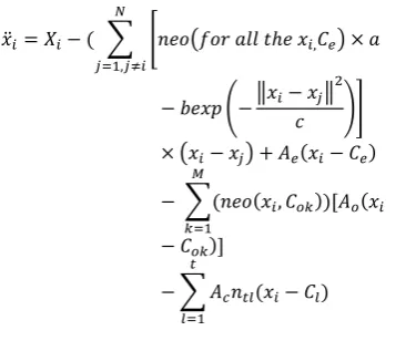
𝑥̈𝑖= 𝑋𝑖− ( ∑ [𝑛𝑒𝑜(𝑓𝑜𝑟 𝑎𝑙𝑙 𝑡ℎ𝑒 𝑥𝑖,𝐶𝑒) × 𝑎 𝑁
𝑗=1,𝑗≠𝑖
− 𝑏𝑒𝑥𝑝 (−‖𝑥𝑖− 𝑥𝑗‖
2
𝑐 )]
× (𝑥𝑖− 𝑥𝑗) + 𝐴𝑒(𝑥𝑖− 𝐶𝑒)
− ∑(𝑛𝑒𝑜(𝑥𝑖, 𝐶𝑜𝑘))[𝐴𝑜(𝑥𝑖 𝑀
𝑘=1
− 𝐶𝑜𝑘)]
(8)
In the above equation, the first term represents the sum of unsteady factors. The second term gives the sum of potential functions used to establish gathering and guarantee no collision between the members.
In this equation, a represents tendency toward gathering, c and b are repulsive agents to guarantee no collision between members and also between members and obstacles, and Ae is the attractive agent toward the target point. These values are designed and selected subject to the following constraints: b > a, a, b, c, > 0, and Ae > 0. Ce represents the coordinates of the target point toward which the members will move.
The designed algorithm should also be able to guarantee no collision between the swarm members and obstacles along the path. In this section, the neighborhood of each obstacle is estimated by a circle. In this case, safe motion is guaranteed when members do not collie to the circle perimeter. In order to provide safe movement, each obstacle is considered as a circular object located within a larger circle with the same center as that of the smaller one. The considered algorithm is designed in such a way that, whenever a swarm member locates on the larger circle, a repulsive agent is activated to guide the member outward the large circle. In order to achieve optimal performance of the designed algorithm, the system is equipped with a switch which is activated should a member falls within the area of the circle, guiding the member outward the circle, with the repulsive agent deactivated once no member is in the circle. This is represented by the third parameter in right-hand side of Equation (8).
Figure 1. Final location of members of a 20-member swarm following 600 steps [11].
Initial position of each member is specified by a hollow circle. As can be observed, under no collision with one another and in absence of any obstacle, the swarm members of different initial locations start to move toward one another. Once gathered at points near the swarm center, the swarm members move toward the target while maintaining the developed arrangement. In this way, since the members should always keep gathered close to one another according to the applied constraints, they are left with limited motion paths to reach the target.
2. Design of optimal stability algorithm for swarm motion
As was mentioned before, the aim of the present paper was to optimize the designed a stability algorithm similar to the one presented in Equation (8). In the mentioned research and similar studies, swarm members motion algorithm is commonly designed in such a way that, the members begin with gathering in a particular area and then move toward the target; i.e. the mission is undertaken once all of the members are gathered in the vicinity of the target [11-15].
Despite numerous advantages of the algorithms designed using this method, those tend to force swarm particles to move long distances. In addition, the constraint upon which the members shall move close to other members can incur motion space limitations in many missions. This is frequently observed in robot swarm motion in small spaces or movement in spaces constraining many obstacles.
This is while, in many of the missions defined for assistant robots, any reduction in the distance traveled by the members is of paramount importance. Moreover, in
many missions, it is observed that swarm members are forced to apportion duties, so that each member is required to cover a particular area of the same target. Surveying operations and similar missions by a swarm of robots are examples of such cases [16-18].
In such cases, in order to optimize the stability algorithm for swarm motion in terms of energy consumption and mission time, one can introduce another parameter into the designed equation of motion for the swarm members. Considered as a potential function, this parameter is designed and applied onto the equation of motion of the swarm members in such a way to eliminate the need for gathering the members around a particular point or the center of the swarm. In this design, certain points are tagged on the target and the introduced term into the equation of motion calculates the distance between each member and the tagged points on the target in real time since the beginning of the swarm motion. As a result, since the start of mission time, each member of the swarm is guided toward the point on the target to which its distance is minimum via an interactive communication to other members of the swarm. This process is simultaneously performed for all members of the swarm, and the information exchange among the members ensures maintaining the swarm properties.
Applying the considered term into the equation of motion, total traveled distance by members to accomplish the mission is expected to reduce. The applied potential function for this purpose is defined as Equation (9).
𝑝𝑜𝑙(𝑥𝑖, 𝐶𝑙) = ∑[
𝐴𝑐
2 ‖𝑥𝑖− 𝐶𝑙‖
2] 𝑡
𝑙=1
(9)
In the above equation, t denotes number of the members in the motion space, Cl is the coordinate of a tagged point on the target, and Ac represents the distance intensity. The gradient 𝑝𝑜𝑙(𝑥𝑖, 𝐶𝑙) will be in the form of Equation (10):
𝜕𝑝𝑜𝑙(𝑥)
𝜕𝑥𝑖
= ∑ 𝐴𝑐𝑛𝑡𝑙(𝑥𝑖− 𝐶𝑙) 𝑡
𝑙=1
(10)
𝑥̈𝑖= 𝑋𝑖− ( ∑ [𝑛𝑒𝑜(𝑓𝑜𝑟 𝑎𝑙𝑙 𝑡ℎ𝑒 𝑥𝑖,𝐶𝑒) × 𝑎 𝑁
𝑗=1,𝑗≠𝑖
− 𝑏𝑒𝑥𝑝 (−‖𝑥𝑖− 𝑥𝑗‖
2
𝑐 )]
× (𝑥𝑖− 𝑥𝑗) + 𝐴𝑒(𝑥𝑖− 𝐶𝑒)
− ∑(𝑛𝑒𝑜(𝑥𝑖, 𝐶𝑜𝑘))[𝐴𝑜(𝑥𝑖 𝑀
𝑘=1
− 𝐶𝑜𝑘)]
− ∑ 𝐴𝑐𝑛𝑡𝑙(𝑥𝑖− 𝐶𝑙) 𝑡
𝑙=1
(11)
3. Simulation and theoretical results
In order to investigate the results of the designed optimal stability algorithm, a swarm composed of two members was considered. Accordingly, behavior of this swarm in moving toward certain points on a hypothetical target is two-dimensionally simulated using Equation (11). The parameters used in this simulation are presented in Table 1.
Table 1. The values used in the simulation.
Parameter Name Value
Attraction to target 𝐴e 1
Repulsion from obstacle 𝐴o 30
Distance intensity 𝐴c 1
Collision avoidance C 0.8
Collision avoidance B 20
Aggregation tendency A 1
Damping coefficient K 5
The obstacles along the motion path were assumed as circles of R0 radius. In this simulation, equation of motion of the swarm was solved using fourth-order Runge-Kutta method with a step size of 0.05. The two coordinates 𝐶𝑒1= [−9 − 6] and 𝐶𝑒2= [−5 − 8] were
considered as two tagged points on a hypothetical in-plane target.
Initial positions of the members were selected arbitrarily in small distance to one another. For all members, initial velocity was considered as zero. The swarm members were simulated for 600 steps. Location of the swarm members are denoted by cross marks while the traveling path of each member is represented by a black line. Following 100 steps of simulation, the swarm members moved as shown on Figure 2.
In the beginning of the simulation, the members tend to diverge from one another due to the repulsive force to guarantee no collision among them. As is shown in
Figure 2, around the existing obstacles, the swarm members tended to follow different motion paths. Next, considering the constraint considered in the swarm equation of motion, each member moved toward the tagged point on the target to which its distance was minimal based on the knowledge of the location of other members and knowing its distance to all of the points tagged on the target.
Figure 3 shows how members moved following 300 steps of simulation. As can be observed, while moving to the corresponding point on the target, each member guarantees no collision to other obstacles.
Figure 4 shows final position of the swarm members based on the simulation of the designed algorithm. As expected, following the end of simulation steps, the members were located at 𝐶𝑒1= [−9 − 6] and 𝐶𝑒2=
[−5 − 8] , respectively. Comparing members’ motion on Figures 2-4 to that on Figure 1 indicates that, implementation of the optimized stability algorithm not only guarantees an interaction among swarm members and satisfies no collision among the members and also between members and obstacles along the motion path, but also eliminates the need for having the swarm members gathered around some points near the center of the swarm as the swarm moves toward the target. As a result, depending on their initial positions, each of the swarm members enjoys higher freedom for moving toward the target. In addition, considering the elimination of the need for gathering early in the beginning of the motion, the mission can be accomplished at faster pace.
In many applications, robots may happen to be located at various initial coordinates and distances to one another. In order to evaluate performance of the designed algorithm in such a case and further verifying the algorithm, swarm members’ motion was simulated once more with various initial coordinates. For instance, the members were assumed to be initially located at 𝑂1=
[−10 0]and 𝑂2= [9 9], respectively, with the location
Figure 2. Simulation of swarm motion following 100 steps.
Figure 3. Simulation of swarm motion following 300 steps.
Figure 4. Simulation of swarm motion following 600 steps.
Furthermore, in order to consider more complicated conditions in terms of position for the swarm members, initial position of one of the swarm members was set to a point close to the obstacles along the motion path 𝑂1=
[5 4], with the position of the second member set at 𝑂2=
[−10 − 8]. The results obtained following 600 steps of simulation on this case are shown in Figure 5.
As can be observed, the paths followed by the swarm members indicate that, the member which was initially close to obstacle begins with attempting to follow the
path along which no collision to obstacles is guaranteed. Continuing with the motion, the designed algorithm guides this member toward the tagged target point to which its distance is minimal. The other swarm member is guided toward the closer target point right from the beginning of the simulation time. As such, the objective of the designed algorithm is also satisfied in these conditions.
Figure 5. Simulation of swarm motion with different initial coordinates for robots
Figure 6. Simulation of swarm motion with different initial coordinates for robots.
4. Future Works
two-member swarm shown in figure 7 with characteristics of table 2 is considered for this reason [19-22].
Figure 7. Designed and manufactured quadrotor [19].
Calculations are shown that each quadrotor can be considered as a point mass regarding some assumptions. Having equations of motion of designed algorithm, each quadrotor can be accepted as a swarm member. Results of applying the designed algorithm on two members swarm moving toward targeted points on space would be published in future.
Table 2. characteristics of manufactured quadrotor [19].
Name Specification
Motor Type DJI2312 (18 A)
Rotor Dimension 10 × 45cm
Battery Type Lithium-ion battery (3
cells/4200 mAh) Acceleration sensor
Type LSM303D (14 bits)
Gyroscope Type MPU6050 (Tri-axial)
Take-off weight <1200g
Maximum Flight
Velocity 10 m/s
Data sample rate 200-400
Filter type Kalman filter
5. Conclusion
In the present paper, designing an optimal motion stability algorithm for a swarm of robots moving toward particular points on an assumed target was presented.
Considering the results of similar researches, equation of motion for swarm members was developed to guarantee no collision between the members and also the members and obstacles along the path. The ultimate goal was to optimize the designed algorithm in terms of energy consumption and motion time. Regarding many missions defined for swarms of robots needed to locate the swarm members at different points on a target, a potential function was further introduced into the equation of motion. The applied potential calculates the
distance between each member and the desired point on the target and also the distance between different members. This function acts in a way that, not only the members interacted with one another along the motion path, but also, calculating the mentioned distances, the algorithm guides the member to a desired point on the target at shortened distance.
Therefore, the need for a premature gathering of the swarm members before moving toward the target seen in many similar researches was eliminated. Providing the members with larger maneuver space optimizing mission time and energy consumption is done by the swarm member.
Following, the designed algorithm was simulated for a swarm containing two members and the results were presented in the form of 2D plots. The results obtained from the simulations are shown that each robot can work with other robots to cover a particular zone, by dividing the targeted area into several intervals. As a result, the need of movement of all swarm members toward the desired points on the target, or being gathered on a particular point before moving toward the target is eliminated.
In conclusion, the swarm members travel shorter distances to reach their predefined target points. This can reduce the time of mission accomplishment while optimizing of energy consumption. This algorithm can be used in various applications such as photography, surveying, rescue operations, and object transportation by assistant robots.
References
[1] G. Flake, The Computational Beauty of Natur, Cambridge University, MIT Press, (1999).
[2] S. Kazadi, Swarm engineering, Ph.D. thesis, California Institute of Technology, (2000).
[3] G. Beni, J. Wang, Swarm Intelligence in Cellular Robotics Systems. NATO Advanced Workshop on Robots and Biological System, (1989).
[4] C.W. Reynolds, Flocks, herds, and schools: A distributed behavioural model, Comp, ACM SIGGRAPH computer graphics, California (1987). [5] A. Kushleyev, D. Mellinger, V. Kumar, Towards A
Swarm of Agile Micro Quadrotor, GRASP Lab, University of Pennsylvania, USA, (2013).
[6] A.M. Naghsh, A. Tanoto, Analysis and design of human-robot swarm interaction in firefighting, The 17th IEEE International Symposium on Robot and Human Interactive Communication, (2008).
[8] A .Mong, S. Loizou, Stabilization of Multiple Robots on Stable Orbits via Local Sensing. IEEE International Conference on Robotics and Automation, (2007).
[9] H. Hashimoto, S. Aso, S. Yokota, A. Sasaki, Cooperative Movement of Human and Swarm Robot Maintaining Stability of Swarm. The 17th IEEE International Symposium , (2008).
[10] V. Gazi. On Lagrangian Dynamics Based Modelling of Swarm Behaviour. Department of Electrical and Electronics Engineering, Istanbul Kemerburgaz University, Turkey, (2013).
[11] A. Ghafari, A. Khodayari, A. Poormahmoodi, Providing an algorithm based on unwillingness to accumulate in the two-dimensional movements of Swarm robots, 24th Annual International Conference on Mechanical Engineering, Iran, (2016).
[12] A. Poormahmoodi, A. Ghaffari, A. Khodayari, Stability pattern of Movements for Swarm Robots. M.Cs thesis, South Tehran Branch, Islamic Azad University, Iran, (2016).
[13] Z. Chen, H. Liao, T. Chu, Aggregation and Splitting in Self-Driven Swarms. Phisica A, Elsevier, (2012). [14] M. Brambilla, E. Frante, M. Birattari, Swarm Robotics: a Review From the Swarm Engineering Prespective. Springer. Swarm Intell, (2013). [15] S. Chui, X. Wang, J. Geng, Intelligent Swarm
Analysis on Aggregation Based Optimal Fuzzy Controller. Controll and Decision Conference , IEEE, China, (2008).
[16] J. Rothermich, I. Ecemiş, P. Gaudiano, Distributed Localization and Mapping with a Robotic Swarm. Springer Berlin Heidelberg, Germany, (2004). [17] V. Kumar, F. Sahin, Cognitive Maps in Swarm
Robots for the Mine Detection Application. Systems, Man and Cybernetics, IEEE, (2003).
[18] J. Kim, J. Wook, J. Seo, Mapping and Path Planning Using Communication graph of Unlocalized and Randomly Deployed Robotic Swarm. Control, Automation and Systems (ICCAS), (2016).
[19] A. Khodayari, A. Ghafari, H. Khodayari, Design, construction and validation of a quadrotor with the aim of using as a swarm member, 25th Conference of Mechanical Engineering, Tarbiat Modarres University, Iran, (2017).
[20] H. Khodayari, Designing of an Optimal Fuzzy Controller Using Linear Quadratic Regulator Method for a Quad-Rotor. MSc thesis, Department of aerospace engineering, Science and Research branch, Azad University, Iran, (2013).
[21] F. Pazooki, H. Khodayari, Attitude stability optimization of a quadrotor with a fuzzy controller.
13th conference of aerospace community of Iran, Tehran University, Iran, (2014).
[22] H. Khodayari, F. Pazooki, Designing an optimal fuzzy controller with LQR method for controlling the attitude of quadrotor. The International Society of Mechanical Engineering Conference (ISME), Iran, (2014).
Biography
Houri khodayari was born in Iran. She received her B.Sc. and M.Sc. degree in Aerospace engineering from Science and Research Branch, Islamic Azad University, in 2010 and 2013 respectively. She is currently a Ph.D. candidate of Aerospace engineering at Science and Research Branch, Islamic Azad University, Tehran, Iran. Her research interests include flight dynamics and control, robotics, and control of unmanned aerial robots.
Farshad Pazooki was born in Iran. He received his Ph.D. degree in Aerospace Engineering from Science and Research Branch, Islamic Azad University in 2008. He is currently an assistant professor in the faculty of Aerospace Engineering at Science and Research Branch, Islamic Azad University, Tehran, Iran. His research interests include flight dynamics and control and adaptive control of flight systems.
![Figure 1. Final location of members of a 20-member swarm following 600 steps [11].](https://thumb-us.123doks.com/thumbv2/123dok_us/8945069.1854437/4.612.67.266.74.260/figure-final-location-members-member-swarm-following-steps.webp)
![Table 2. characteristics of manufactured quadrotor [19].](https://thumb-us.123doks.com/thumbv2/123dok_us/8945069.1854437/7.612.84.253.94.220/table-characteristics-of-manufactured-quadrotor.webp)
