Hardware Implementation of a Novel Image Compression Algorithm

(1)

University of New Orleans University of New Orleans

ScholarWorks@UNO

University of New Orleans Theses and

Dissertations Dissertations and Theses

1-20-2006

Hardware Implementation of a Novel Image Compression

Algorithm

Vikas Kumar Reddy Sanikomm

University of New Orleans

Follow this and additional works at: https://scholarworks.uno.edu/td

Recommended Citation Recommended Citation

Sanikomm, Vikas Kumar Reddy, "Hardware Implementation of a Novel Image Compression Algorithm" (2006). University of New Orleans Theses and Dissertations. 1032.

https://scholarworks.uno.edu/td/1032

(2)

HARDWARE IMPLEMENTATION OF A NOVEL IMAGE

COMPRESSION ALGORITHM

A Thesis

Submitted to the Graduate Faculty of the University of New Orleans

in partial fulfillment of the requirements for the degree of

Master of Science in

Engineering

by

Vikas Kumar Reddy Sanikommu

B.S.,Jawaharlal Nehru Technological University,Hyderabad,2002

(3)

ACKNOWLEDGEMENTS

I would like to express my gratitude to my Advisor, Dr Dimitrios Charalampidis, for

his support and timely advice through out my research. I appreciate and value his consistent

feedback on my progress, which was always constructive and encouraging.

I would also like to express my sincere thanks to the other committee members, Dr.

Vesselin Jilkov and Prof. Kim D Jovanovich for their willingness to be on my thesis

committee and helping me in the dire moments of Katrina. Their invaluable suggestions and

insightful comments have made my work more presentable. I would really like to appreciate

them for allowing me get some of their valuable time in the time of Katrina for my defence.

(4)

LIST OF TABLES

Comparison between Single Structure and Adaptive Architecture 45

(7)

LIST OF FIGURES

Figure 2.1 (a) Predictive Coding Encoder. 10

Figure 2.1(b) Predictive Coding Decoder. 10

Figure 3.1 Block Diagram of JPEG encoding. 15

Figure 3.2 Block Diagram of JPEG decoding. 16

Figure 3.3 Zig-Zag Sequence for Binary Coding 17

Figure 5.1 Encoding Phase of the Proposed Algorithm 24

Figure 5.2 Decoding Phase of the Proposed Algorithm 25

Figure 5.3 Weights and Coefficient Estimation Block 29

Figure 5.4 Decoding Phase of a Single-NN with a Single Stage 33

Figure 6.1 Code Composer Studio Architecture from TI Documentation 38

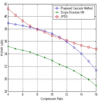
Figure 7.1 PSNR Values for reconstructed Lena Image at Different Compression Ratios 46

Figure 7.2 PSNR Values for reconstructed Pepper Image at Different Compression Ratios 47

Figure 7.3 PSNR Values for reconstructed Baboon Image at Different Compression

Ratios 48

Figure 7.4(a) Graphical Display of the Original Lena Image. 49

Figure 7.4(b) Reconstructed Lena Image at CR 8:1 by Single-Structure NN. 50

Figure 7.4(c) Reconstructed Lena Image at CR 8:1 by Proposed Architecture. 50

(8)

ABSTRACT

Image-related communications are forming an increasingly large part of modern

communications, bringing the need for efficient and effective compression. Image

compression is important for effective storage and transmission of images. Many techniques

have been developed in the past, including transform coding, vector quantization and neural

networks. In this thesis, a novel adaptive compression technique is introduced based on

adaptive rather than fixed transforms for image compression. The proposed technique is

similar to Neural Network (NN)–based image compression and its superiority over other

techniques is presented

It is shown that the proposed algorithm results in higher image quality for a given

compression ratio than existing Neural Network algorithms and that the training of this

algorithm is significantly faster than the NN based algorithms. This is also compared to the

JPEG in terms of Peak Signal to Noise Ratio (PSNR) for a given compression ratio and

computational complexity. Advantages of this idea over JPEG are also presented in this

(9)

CHAPTER 1 INTRODUCTION

Digital images contain large amounts of data. Therefore, a high image quality implies that the

associated file size is large. For the sake of storage and transmission over channels at high

efficiency, a high quality, highly compressive algorithm for image compression is at demand.

Despite the existence of image compression standards such as JPEG and JPEG 2000, image

compression is still subject to a worldwide research effort. Image compression is used to

minimize the amount of memory needed to represent an image. Images often require large

number of bits to represent them, and if the image needs to be transmitted or stored, it is

impractical to do so without somehow reducing the number of bits. The problem of transmitting

or storing an image affects all of us daily. Namely, TV and fax machines are both examples of

image transmission, and digital video players and web pictures are examples of image storage.

By using data compression techniques, it is possible to remove some of the redundant

information contained in the images, requiring less storage space and less time to transmit.

Another issue in image compression and decompression is increasing processing speed, without

losing the image quality especially in real-time applications.

Many compression techniques have been developed in the past, including transform coding,

vector quantization, pixel coding and predictive coding. Most recently, Neural Network based

techniques have being used for compression. Next, the compression types are discussed.

1.1 Lossless Compression

These techniques generally are composed of two relatively independent operations: (1) devising

(10)

(2) coding the representation to eliminate coding redundancies. Typical schemes are based on

Huffman encoding. They normally provide compression ratios of 2 to 10 [6].

1.2 Lossy Compression

Unlike the Lossless Compression approaches, Lossy encoding is based on the concept of

compromising the accuracy of the reconstructed image in exchange for increased compression.

Many lossy encoding techniques are capable of reproducing recognizable images from data that

have been compressed by more than 30:1, and images indistinguishable from the originals at 10:1

to 20:1 [6].

Transform-based coding techniques have proved to be the most effective in obtaining large

compression ratios while retaining good visual quality. In low noise environments, where the bit

error rate is less than 10-6, the JPEG [3]-[4] picture compression algorithm, which employs

cosine-transforms, has been found to obtain excellent results. However, an increased number of

real-time applications require that compression be performed in highly noisy environments with

high bit error transmission rates [12]. In this cases, JPEG and other compression techniques

involving fixed transforms are not capable of maintaining high image quality.

Many recently developed techniques such as the wavelet Based, JPEG2000 technique, show

some adaptability. With the involvement of Neural Networks in image compression, adaptive

techniques have evolved [1]-[8]. Neural Networks have been proved to be useful in image

compression because of their parallel structure, flexibility, robustness under noisy conditions and

simple decoding [15]-[20]. However, there is a reduction in the quality of the decompressed

image for the same compression efficiency.

Compression using Neural Networks suffers from several drawbacks, including:

(11)

(2) High Computational complexity,

(3) Moderate Compression ratio and

(4) The reconstructed image quality is training dependent.

These techniques involve Single Structure and Parallel Structure Neural Network architectures.

Parallel structures result in a higher decoded image quality than the single structured techniques.

This thesis introduces a different approach to adaptive image compression, which overcomes the

above drawbacks. This architecture consists of a cascade of simple adaptive linear units. This

technique is similar to the parallel NN technology in that image blocks can be encoded by

different parts of the architecture. An image block is encoded using only a subset of stages and

hence the total number of learning parameters is small with their estimation happens to be faster

than that of NN techniques. This makes training a part of coding. The technique adapts to the

content in order to calculate a set of transforms that code the image in a block manner similar to

JPEG. The adaptive nature of this technique allows the extraction of the image information from

(12)

CHAPTER 2 TECHNIQUES OF IMAGE COMPRESSION

As mentioned earlier, image compression techniques can be classified mainly as lossless and

lossy.

2.1 Lossless Compression:

Lossless compression is the method in which the original data can be preserved after

reconstruction without any loss, which means that the decompressed image looks nearly the same

as the original image. These methods are preferred where high value content is required. Some of

such applications include medical imaging or images made for archival consent. Some of the

lossless coding techniques are:

• Run length coding

• Huffman coding

• Entropy coding

2.1.1 Run length Coding:

Run length encoding (RLE) is a sequential data compression technique used to reduce the

size of a repeating string of characters. This repeating string is called a run. RLE encodes a run of

symbols into two bytes, a count and a symbol. RLE compresses any type of data regardless of its

content but the content of data to be compressed affects the compression ratio.

Consider a character run of 16 characters as:

‘aaaccccccvvvtttt’

Which normally would require 16 bytes to store but with RLE this would only take 8 bytes of

data to store, the count is stored as the first bit and the symbol as the second bit which is:

(13)

In this case RLE yields a compression ratio of 16:8 that is 2:1.

Images with repeating grey values along the rows (or columns) can be compressed by storing

runs of identical grey values as:

Grey value 1 Repetition 1 Grey value 2 Repetition 2

Run length coding is fast and can easily be implemented but the compression is very limited as it

requires a minimum of two characters worth of information to encode a run.

2.1.2 Huffman coding:

Huffman coding is the most popular technique for removing coding redundancy. This code

provides a variable length code with minimal average code–word length (least possible

redundancy). This yields the smallest possible number of code symbols per source symbol. The

first step in this technique is to create a series of source reductions by sorting the message

symbols under consideration in the increasing order and combining the lowest probability

symbols into a single symbol until the entire message is finished.

The second step in this technique is to code each reduced symbol starting with the smallest and

back to the original symbol. Example for this procedure is:

Original Source Source Reduction

Sym. Prob. Code 1 2 3 4

V2 0.4 1 0.4 1 0.4 1 0.4 1 0.6 0

V6 0.3 00 0.3 00 0.3 00 0.3 00 0.4 1

V1 0.1 011 0.1 011 0.2 010 0.3 01

V4 0.1 0100 0.1 0100 0.1 011

V3 0.06 01010 0.1 0101

(14)

2.1.3 Entropy coding:

The implementation of this method is a variable-to-fixed length code. This is an adaptive based

technique. This technique uses the previous data to build a dictionary. This dictionary consists of

all the strings in a window from the previously read data stream. The window is divided into two

parts fixed-size window and look-ahead buffer. The fixed-size window consists of large blocks

of decoded data and the look-ahead buffer consists of data read in from the data read but not yet

encoded. The data in the buffer is then compared with the data in the fixed-size window. In the

dictionary based method, the phrases are replaced with the tokens and if the number of bits in the

token are less than the number of bits in the phrase compression occurs. Consider the following

example:

Implementing in code composer studio Code composer studio is

Fixed-size window of previously read Look –ahead buffer (20 bytes)

data (32 bytes)

In this example, if any matches are found then a token is sent to the output stream describing the

match. When this symbol is matched, the data is shifted by an amount equal to the length of the

symbol represented by the previous token. Data is pushed out of the token and new data is read

into the buffer as shown:

Implementing in code composer studio , is

Here the code composer studio is added to the dictionary and every time it is seen after this a

token is passed in the phrase.

The three items taken care of in the token are:

(15)

• The length of the phrase

• The first symbol in the look-ahead buffer that follows the phrase

• The idea of this method is to build a dictionary of strings while encoding. The encoder

and decoder start with an empty dictionary in this method. The dictionary is added with

each character as long as it matches a phrase in the dictionary. The compression of this

method is poor but, as the strings is re-seen and replaced in the dictionary the

performance increases.

2.2 Lossy compression:

Lossy encoding is based on the concept of compromising the accuracy of the reconstructed

image in exchange for increased compression. Lossy techniques provide far greater compression

ratios than lossless techniques. In many applications, the exact restoration of the image is not

always necessary. The restored image can be different to the original without the differences

being distinguishable by the human eye. Some of the lossy coding methods are:

• Vector Quantization

• Transform Coding

• Fractal Compression

2.2.1 Vector Quantization:

Quantization is the procedure of approximating the continuous values with discrete values. The

goal of quantization usually is to produce a more compact representation of the data while

maintaining its usefulness for a certain purpose. There are two basic quantization types, namely

scalar quantization and vector quantization. In scalar quantization, both the input to and output

(16)

are called codewords. Scalar quantization is not optimal as successive samples in an image are

usually correlated or dependent, thus it has been observed that a better performance is achieved

by coding vectors instead of scalars. Several vector quantization schemes exist to take advantage

of different characteristics in the image.

In image compression using vector quantization, the procedure followed for codebook design is

one of the essential parts of the technique, and directly affects the compressed image quality.

First, a training image is split into blocks, and each block is represented in the form of a vector.

The set of vectors obtained from the training image is called the set of training vectors. The

codebook design procedure uses the training vectors in order to construct the codebook.

Essentially, the codewords are a set of vectors that approximate the larger set of vectors obtained

from the training image.

Let us assuming that training has already been performed, this implies that the codebook has been

obtained. Then, a vector quantizer consists of the following:

(1) The encoder that compares the vectors x extracted from the image to be compressed,

with the codebook vectors. If a vector x is found to be “closest” to one of the

codewords, then the codeword’s corresponding index is assigned to the vector x. The

closeness of a vector to a codeword is defined by a distortion measure. One such

commonly used distortion measure is the Euclidean distance.

(2) The decoder that maps an index back to the corresponding codeword in order to

obtain an approximation of the original vector x.

The standard approach to construct the codebook is by Linde-Buzo-Gray’s algorithm (LBG) [10].

2.2.2 Transform Coding:

In transform coding, a reversible linear transform is used to map the image into a set of transform

(17)

typical transform coding system has four steps: (1) Decomposition of image into sub-images, (2)

Forward transformation, (3) Quantization, (4) Coding.

An N x N image is subdivided into sub images of size n x n (mostly 8 x 8), which are then

transformed; so as to collect as much information into a smaller number of transform

coefficients. The quantization then quantizes the coefficients that contain the least information.

The encoding process ends with the coding of the transformed coefficients. The most famous

transform coding systems are Discrete Cosine Transform (DCT), and Karhunen-Loeve (KLT).

Discrete Transform Coding is preferred over all the transform coding techniques as it involves

less number of calculations. The standard presently accepted, created by the Joint Photographic

Experts Group (JPEG) for lossy compression of images uses DCT as the transformation. More

about the DCT is discussed in the background chapter of this thesis.

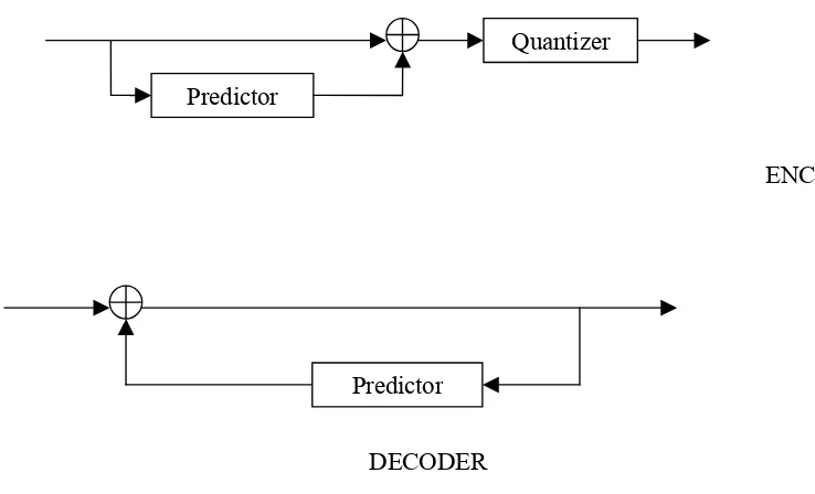
2.2.3 Predictive Coding:

Predictive image coding techniques take advantage of the correlation between adjacent pixels.

This mainly consists of the following three components:

(1) Prediction of the current pixel value

(2) Calculating the prediction error

(3) Modeling the error distribution

The value of the current pixel is predicted based on the pixels that have already been coded. Due

to the correlation property among adjacent pixels in an image, the use of predictor can reduce the

amount of information bits required to represent an image.

In predictive coding also called Differential Coding such as Differential Pulse Code Modulation

(DPCM), the transmitter and receiver process the image in some fixed order. The current pixel is

(18)

current pixel P(x, y) and its predicted value P1(x, y), the prediction error d(x, y), is then

quantized, encoded and transmitted to the receiver. If the prediction is well defined, then the

distribution of the prediction error is concentrated near zero and has lower first order entropy

than the entropy of original image.

The design of this predictive coding scheme involves two main stages, predictor design and

quantizer design. Although general predictive coding is classified into AR, ARMA etc,

auto-regressive model has been applied to image compression. Predictive coding can further be

classified into Linear and Non-linear AR models. Non-linear predictive coding, however, is very

limited due to the difficulties involved in optimizing the coefficients extraction to obtain the best

possible predictive values.

ENCODER

DECODER

Fig 2.1 Predictive Coding (a) Encoder (b) Decoder Quantizer

Predictor

(19)

2.2.4 Fractal Coding:

Fractal Coding is a lossy compression method which uses fractals to compress images.

Fractal parameters, like fractal dimension, lacunarity, and others provide efficient methods of

describing imagery in a highly compact fashion for both intra and inter frame applications.

This method is used to compress the natural scenic images where certain parts of the image

resemble the other parts of the same image. Fractal compression is much slower than the

(20)

CHAPTER 3 IMAGE COMPRESSION USING JPEG STANDARD

JPEG stands for Joint Photographic Experts Group (collaboration between ITU and ISO) which

is a group of experts working with the gray scale and color images. JPEG corresponds to the

international standard for digital compression of continuous tone (multilevel) still images. JPEG

compression algorithms involves eliminating redundant data, the amount of loss is determined by

the compression ratio, typically about 16:1 with no visible degradation. For more compression

where noticeable degradation is acceptable compression ratios of up to 100:1 can be employed.

The JPEG algorithm performs analysis of image data in such an order to generate an equivalent

image which can be represented in a much compact form and needs less space to store. JPEG has

two schemes of compression the lossy JPEG, the compressed image when decompressed back is

not the same here and lossless JPEG compression does not lose any image data when

decompressed back. JPEG usually works by discarding the data information a human eye cannot

recognize like slight changes in color are not perceived by the image as the changes in the

intensity are. Due to this fact we can see that JPEG compresses color images more efficiently

than the gray scale images. Thus, most multimedia systems use compression techniques to handle

graphics, audio and video data streams and JPEG forms the important compression standard with

various compression techniques as building blocks.

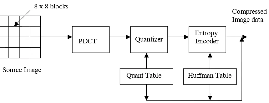
3.1 JPEG Image Compression System:

The main components of the image compression system are:

• Source encoder (DCT based)

• Quantizer

(21)

In the image compression algorithm the image is first split into 8x8 non overlapping blocks and

the two-dimensional DCT is calculated for each block. The DCT coefficients are then ordered in

a zigzag pattern so that the coefficients corresponding to the lower frequencies are ordered first.

The DCT coefficients are then quantized. Insignificant coefficients are set to zero and since not

all the coefficients are used a delimiter are used to indicate the end of required coefficient

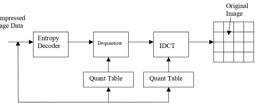
sequence in a block. The coefficients are then coded and transmitted. The JPEG receiver or

decoder then decodes the quantized DCT coefficients, performs inverse two-dimensional DCT of

each block and then puts the blocks together into an image.

3.2 Discrete Cosine Transformation (DCT):

The DCT is closely related to the DFT in that they can be considered to perform the same task of

converting a signal into elementary frequency components. DCT is superior to DFT in that DCT

is real valued and provides better approximation of the signal with fewer coefficients. DCT helps

separate the image into parts of differing importance.

A two-dimensional DCT of an N1xN2 matrix is defined as follows:

The series form of the 2D discrete cosine transform (2D DCT) pair of formulas is

[

] [ ] [ ]

[

]

(

)

(

)

_











Π

+













Π

+

=

∑

−₌

∑

₌− 2 2 2 1 1 1 1

0 1 2

1 0 2 1 2 1

2

1

2 cos

2

1

2 cos

,

2 2 1 1

N

k

n

N

k

n

x

k

c

k

c

k

X

_nN _nN

for k₁=0,1,2,...N₁−1 and k₂ =0,1,2,...N₂ −1 (1)

[

]

[

] [

]

(

)

(

)

_











Π

+













Π

+

=

∑

−₌

∑

₌− 2 2 2 1 1 1 2 1 1

0 1 2

1 0 2 1

2

1

2 cos

2

1

2 cos

,

2 2 1 1

N

k

n

N

k

n

k

X

k

c

n

c

_kN N_k

(22)

α[k] is defined as:

α[k] =      

− =

=

1 ,...., 2 , 1 2

0 1

N k

for N

k for N

(3)

Where the input image is N1×N2, x[n1,n2] is the intensity of the image and X[k1,k2] is the DCT

coefficient in the k1th row and k2th column.

Fig 3.1 JPEG encoder Block Diagram Quant Table

PDCT Quantizer

Entropy Encoder

Huffman Table Source Image

8 x 8 blocks

(23)

Fig 3.2 JPEG Decoder Block Diagram

Each 8x8 block is compressed into a data stream in the DCT encoder and because the adjacent

image pixels are highly correlated the forward DCT concentrates most of the data in the lower

spatial frequencies. The output from the FDCT is then uniformly quantized by using a designed

quantization table. For a typical 8x8 sample block from a source image, most of the spatial

frequencies have zero or near-zero amplitude and need not be encoded. The DCT introduces no

loss to the source image samples it simply transforms them to a domain in which they can be

more efficiently encoded. The output from the FDCT (64 DCT coefficients) is uniformly

quantized with a designed quantization table. At the decoder the quantized values are multiplied

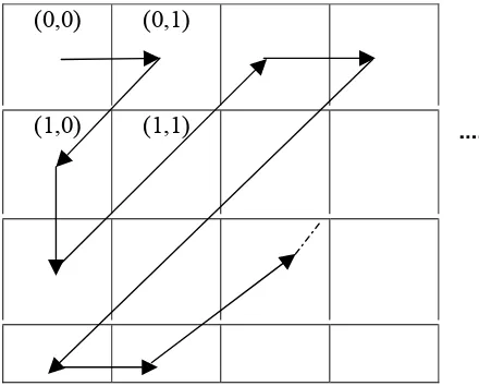
with the quantization table elements to retrieve the original image. After quantization the

coefficients are placed in a ‘zig – zag’ manner which helps in entropy coding by placing the

low-frequency non-zero coefficients before high low-frequency coefficients. The DC coefficients are

differently encoded. The zig zag sequence is as shown below: Entropy

Decoder Dequantizer IDCT

Quant Table Quant Table Compressed

Image Data

(24)

(0,0) (0,1)

(1,0) (1,1)

Fig 3.3 Zig – Zag Sequence for Binary Coding

3.3 Quantization:

Each output from the DCT is divided by a quantization coefficient and rounded to an integer to

further reduce the values of the DCT coefficients. Each of the DCT output coefficients has its

own quantization coefficient with the higher order terms having the larger quantization

coefficients which make the higher order coefficients quantized more profoundly than the lower

order coefficients. The quantization table is sent along with the compressed data to the decoder.

The quality factor set affects the amount of quantization performed on the image. Too much and

too little quantization effect the image by making it either blurry or causes loss of information.

3.4 Entropy Encoder:

Entropy coding achieves additional compression by encoding the quantized DCT coefficients

based on their statistical characteristics. Huffman coding or Arithmetic coding can be used.

Arithmetic compression involves mapping every sequence of pixel values to a region on an

(25)

variable precision (number of bits). Less common sequences are represented with a binary

fraction of higher precision.

3.5 Differential Pulse Code Modulation (DPCM):

In a DPCM model a certain number of pixels in the neighborhood of the current pixel are

considered to estimate/predict the pixel’s value. In the sense the coding of the DC coefficient is

done by the differential between the quantized DC coefficient of the current block and the

quantized DC coefficient of the previous block. The inverse DPCM returns the current DC

coefficient value of the quantized block being processed by summing the current DPCM code

with the previous DC coefficient value of the previous quantized block.

3.6 RLE:

The AC coefficients usually contain a number of zeros. Therefore RLE is used to encode these

zero values by keeping the skip and the value where skip is the number of zeros and value is the

next non-zero component.

(26)

CHAPTER 4 NEURAL NETWORK FOR IMAGE COMPRESSION

Artificial Neural Networks are hardware or software systems based on the simulation of a

structure similar to that a human brain has. The important element here is the information

processing unit which is composed of one or more layers of groups of processing elements called

neurons. The neurons are connected in such a way that the output of each neuron goes as input to

one or more neurons, to solve the problems. There are three layers in each Neural Network

system: Input layer, Hidden layer and output layer. The input layer and the output layer are of the

same size while the hidden layer is smaller in size. The encoded input goes to the hidden layer

and then to the output layer where it is processed (decoded) in the network of neurons. The ratio

of size of input layer and the intermediate hidden layer is the compression ratio. In most neural

network image compression techniques importance is given to the quality of the image for a give

compression ratio. But image compression using neural network techniques is considered

because of certain advantages of NN such as: their ability to adaptability to learn from the data

given for the training and faster decoding. The process of Neural Networks can be divided into:

the arrangement of neurons into various layers, deciding the type of connection between neurons

inter-layer and intra-layer, finding the way the output is produced from the neurons depending on

the input received the learning for adjusting the weight connections.

4.1 Connection Between Neurons:

The type of connection between neurons can be: inter–layer, connection between two layers and

intra-layer, connection between neurons in one layer. Inter-layer connections can be classified

into: fully connected where each neuron from a layer is connected to each neuron from another

(27)

in another layer; feed-forward where neurons in a layer sends output to neurons in another layer

but don’t receive any feedback which makes the connection between neurons one-directional;

bi-directional where there is a feedback from the neurons in the other layer when they send their

output back to the first layer; hierarchical where the neurons in a layer are connected only to the

neurons in the next neighboring layer; resonance-two directional connection where neurons

continue to send information between layers until a certain condition is satisfied. Neural

Networks can also be classified based on the connection between input and output: auto

associative, input vector is same as the output. These can be used in pattern recognition, signal

processing, noise filtering, etc; heteroassociative, output vector differs from the input vector.

4.2 Basic Principles of NN Architectures:

The value of the input to a neuron from its previous layer can be computed by an input function

normally called a summation function. This function can simply be said as the sum of weighted

inputs to the neuron. There are also two specific types of inputs in a network: external input

where a neuron receives input from external environment and bias input where a value is sent for

neuron activation controls in some networks. Normally the input to many NNs is normalized.

After the input from the summation function is received the output of a neuron is computed and

sent to the other connected neurons. This output to a neuron is normally computed using a

transfer function which can be a linear or non-linear function of its input. The transfer function is

chosen according to the problem specified. Some of the transfer functions are the step function,

signum function, sigmoid function, hyperbolic-tangent function, linear function, and threshold

(28)

4.3 Learning:

The process of calculation of weights among neurons in a network is called Learning. The

network can be considered by supervised learning and unsupervised learning. In the supervised

learning the network is given with a set of input and a desired output set. The network weights

here are adjusted by comparing these outputs with the desired outputs. In the unsupervised

learning the network is given only a set of input without any desired output set making the

network to adjust the weights by itself to improve the clustering of data. This is commonly used

for pattern recognition and clustering.

Depending on the number of layers Neural Network designs can be: single layered only with the

output layer or multi-layered with one or more hidden layers. A NN can be deterministic where

the impulses to the other neurons are sent when a neuron gets to a certain activation level and

stochastic where it is done by a probabilistic distribution. A NN can also be a static network

where the inputs are received in a single pass and dynamic network where the inputs are received

over a time interval.

Two major techniques of NN for image compression are the single – structure NN technique and

the parallel – structure NN technique.

4.4 Single Structure NN-based Image Compression:

Many approaches have been implemented for a single structure NN like: Basic back –

propagation algorithm, Hebbian Learning based algorithm, Vector Quantization NN algorithm

and Predictive Coding NN algorithm. In this the image is split into J blocks {Bj, j=1, 2… J} of

size M x M pixels. The pixel values in each block are rearranged to form a M2length pattern Cj =

{C1,j, C2,j, . . ., CM2_,_j_{}, where}_j_{= 1, 2, …,}_J₍_C_i_,_j_{is the}_i_th_{element of the}_j_th_{pattern). The input}

(29)

respectively, the average and standard deviation of Cj because the NNs operate more efficiently

when the input is in the range [0, 1]. These patterns are used both as inputs and outputs in the

training of NNs. The NN consists of three layers as said above the input, hidden and the output

with M2_{, H and M}2 _{nodes in each}

.

4.4.1 Training:

The configuration of Neural Networks for the applications in which the parameters of the

network are adjusted such that the network exhibits the desired properties is called training. The

network is trained so as to minimize the mean square error between the output and the input

values to maximize peak signal to noise ratio. Based on the way the weights are updated the

training can be done by online training, the weights here are updated for each input and Batch

wise training, the weights here are updated when a complete batch is input to a neural network.

The Neural Network acts as coder/decoder. The coder consists of input-to-hidden layer weights

v_i_,_k{ i=1,…,M2 and k=1,…,H},and the decoder consists of the hidden-to-output layer weights

w_k_,_m{k =1,…,H and m =1,…,M2} where v_i_,_k is the weight from the ith_{input node to the k}th

hidden node and w_k_,_m is the weight from the kth hidden node to the mth output node.

Compression is achieved by setting the number of hidden nodes smaller than the number of input

nodes and propagation of the patterns through the weights vi,k. Considerable compression is

achieved when the hidden layer nodes are quantized. The coding product of the jth pattern Pj is the

hidden layer output Oj = {O1,j, O2,j, . . ., OH,j}. The set {Oj, mCj,σCj} together with weights wk,m

is sufficient for reconstructing an approximation Cj of the original pattern Cj in the decoding

(30)

4.5 Parallel – Structure NN-based Image Compression:

The parallel structure is considered as a single structure with multiple hidden layers. Four

networks {NETk, k = 1, 2, 3, 4} with different number of hidden nodes (4, 8, 12, and 16) are used

to achieve a compression ratio 8:1 with each NN trained as a single structure NN. Each pattern is

associated with a NETk.It is assumed that the larger the number of hidden nodes of the NN to

which a pattern is assigned, the smaller the associated error 2

j

e = (Λp_j -p_j) ( pΛ_j -

j

p )T_{between the original p}

jand estimated patterns pj

Λ

. It is an iterative procedure after this. At

each iteration the aim is to reduce the total error E2₌∑_e

j2 without changing the compression ratio.

If de2j, k is the error caused due to reassigning pattern pj from NETk to NETk+1 then the error is

reduced by reassigning a pair of patterns. Pattern Pj1is reassigned from NETk1 to NETk1+1 if the

reassignment causes a maximum error decrease de2 ,ki

ji = max (de_jk

2 ,k

j ), and pattern Pj2 is

reassigned from NETk2 to NETk2-1 if this results in a minimum error increase de2_ji_,_ki =

jk min(de2

,k

j ). Iterations continue as long as the error E2 decreases.

This parallel architecture has the advantage of providing better image quality for a given CR than

other methods like JPEG in terms of error E2, including both single and parallel structures.

Coding is faster than previous parallel architectures. But, training is still significantly slow due to

the use of multiple networks. Moreover, the total number of weights is large. Thus, training

cannot be part of the coding process. Thus, the compression quality depends on the training data

(31)

CHAPTER 5 PROPOSED ADAPTIVE ALGORITHM

The novel Image compression technique implemented in this thesis is based on a cascade of

adaptive transforms. The small number and fast estimation of learning parameters make the

training of data, to be a part of encoding process which makes this technique apt for image

compression. This method uses a cascade of adaptive units called adaptive cascade architecture

(ACA). Each unit is equivalent to a feed-forward neural network with a single node at the hidden

layer. The coding is independent of training data. The encoder and decoder of this technique are

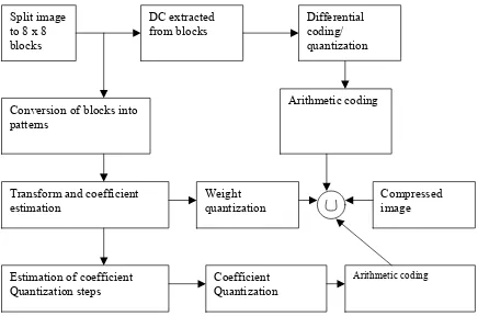
shown in the figures below:

Fig. 5.1 Encoding Phase of the proposed architecture Split image

to 8 x 8 blocks

DC extracted from blocks

Differential coding/ quantization

Conversion of blocks into patterns

Arithmetic coding

Transform and coefficient

estimation Weight quantization Compressed image

Estimation of coefficient

Quantization steps Coefficient Quantization

(32)

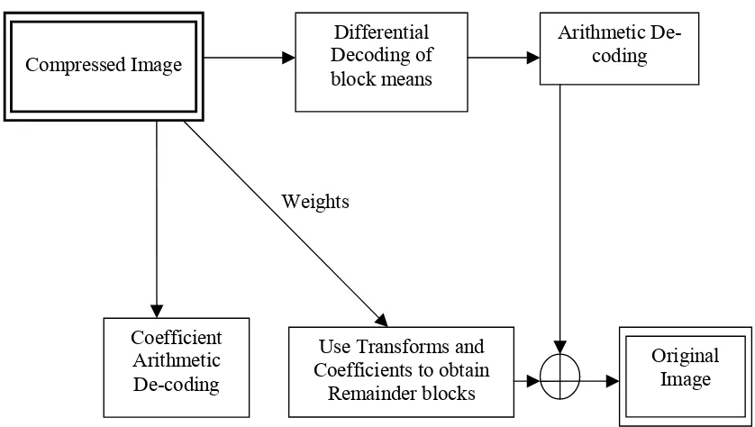
Fig 5.2 Decoding Phase of the proposed algorithm

5.1 Encoding Process:

This section describes the details of each block in the encoder:

Image Splitting into Blocks:

The image is split into J blocks (Bj, j =1, 2, 3… J) of size M×M pixels. Large processing blocks provide a smaller number of transform coefficients but the transform weights, which need to be

stored are increased.

Block means from each block: Compressed Image

Differential Decoding of block means

Arithmetic De-coding

Coefficient Arithmetic De-coding

Use Transforms and Coefficients to obtain

Remainder blocks

(33)

The mean of each block j denoted as mcj contains some significant amount of information it is

extracted from each block.

Differential coding/quantization of mean values:

The DC values of consecutive blocks j and j+1,namely mj and mj+1 are likely to be similar thus

they are differentially encoded: the difference of consecutive mean values dmj = mj+1- mj is

linearly quantized. The number of quantization levels depends on the compression ratio.

Conversion of remainder blocks into patterns:

The pixel values in each non-overlapping block are arranged to form a M2 length pattern Cj =

(C1,j , C2,j , ….., CM2,j ) , where j=1, 2, ….. J ( Ci,j is the ith element of the jth pattern). The input

patterns are defined by Pj = f (Cj ) = ( Cj-mCj ). The transform and coefficient estimators will be

referred to as units. Patterns Pj are used as inputs/desired-outputs to train the first unit.

Weights and Coefficients estimation:

This step is considered as an alterative to DCT, the heart of JPEG. It involves the estimation

of weights and their corresponding coefficients. The output of the first unit’s hidden node

corresponding to the jth pattern is denoted as Oj,k, k=1. The first unit’s estimated weight vector is

denoted by

Wk = [W1,k, W2,k , . . . , WM2,k]; k=1 (4)

This is equivalent to the weight vector between the hidden node and the output layer. Wk is the

kth transform i.e. the ith weight of the kth unit. The weight vector between the input node and the

hidden layer is not required to be implemented. The output coefficient Oj,1 and the weight W1 are

(34)

The first unit’s error patterns are denoted as

ej,1 = [e1,j,1, e2,j,1, ……, eM2,j,1] (5)

These are the difference between the original pj and the estimated patterns p_j

Λ

at the output of the

first unit when the training is complete. ei,j,k is the ith element of the jth error pattern at unit k. If a

set of error patterns at the output of unit k is defined as Rk then only a subset of these error

patterns is used as input/output to train the next unit. This subset Rks consists of S error patterns

esj,k ,j=1,2,…..,S the square sum of whose is larger than a given threshold Q. Rks = { esj,kЄ Rk, esj,k

esj,kT > Q }. Again the second unit’s hidden node output coefficients Oj,2 and weight vectors W2

are stored for the decoding process.

The second unit’s error patterns e2,j are similarly defined as the difference between the actual esj,1

and the estimated error patterns e^sj,1 at the second unit’s output. Only a subset of these new error

patterns e2,j are used as inputs/desired-outputs to train the third unit. This adding and training of

units is repeated until the compression ratio does not exceed a given target. As only a subset of

error patterns trains each unit, the number of outputs Oj,k per unit k is variable. This allows

assignment of image-blocks with larger estimation error to more units, with the same CR.

The threshold Q is defined as

( )

e

CR

M

a

Q

M

i j

j

i













=

∑

=

2

1

1 , , 2

var

1

(6)

From the Equation it can be seen that the threshold Q is proportional to the desired compression

ratio CR. The threshold can be set to a low value because a low compression ratio causes a small

coding error. The threshold is also proportional to the average standard deviation of the error

patterns between the original and the encoded images which is the similarity measure between

(35)

the image blocks. As a result the additional adaptive units are expected to produce a relatively

small coding error and hence the threshold can be ser low. In the Equation a, is a fixed parameter

and is given a value of 1.2 for all the experiments.

The advantage of this adaptive cascade technique over the existing parallel NN architectures is

that total number of weights is relatively smaller and number of hidden node outputs is variable.

The training time is also low because of the low computational complexity of the units. The

algorithm converges in 4-5 iterations by using a set of equations:

Oj,k = Wk Tj,kT/ Wk WkT (7)

Wk = ∑j Oj,k Tj,k / ∑j O2j,k (8)

Tj,k = Pj if k=1

= esj,k-1 otherwise (9)

Equation 7 gives the unit’s optimum hidden layer output coefficients Oj,k given the unit’s

weights. This is the result of minimizing the sum of squares (SSE) between the input and output

patterns.

SSEk =

∑

_

  

 

− 

  

 

−Λ Λ

j

T k j k j k j k

j T T T

T , , , , (10)

Where T j,k Λ

= Oj,kWk, for unit k with respect to Oj,k. Equation (8) gives unit’s optimum unit’s

weights given the hidden layer output coefficients Oj,k. This is the result of minimizing SSEj,k

with respect to Wk. The conditions from which the Equations (7) and (8) are derived are:

(36)

0 , = ∂ ∂ k j k O SSE

and = 0

∂ ∂ k k W SSE (11)

since only the transform weights and the hidden layer output coefficients are needed in the

decoding process it is necessary to find the optimum set {Wk, Oj,k} for each transform unit [c].

The algorithm based on equations (7) and (8) directly gets the sub optimum values for both Wk

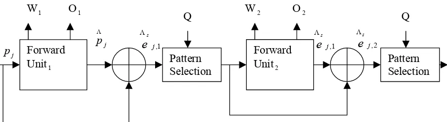
and Oj,k. The weights and coefficient estimation block is as shown in the figure below:

Fig 5.3 Weights and Coefficients estimation Block (Encoding)

Weight Quantization:

After the adaptation the weights are linearly quantized using 256 quantization levels for weight

values in the interval [-1, 1]. Before quantization the weights are normalized so that the

maximum absolute value equals to 1 as shown below:

Wk = Wk/

( )

_i_k

i W,

max (12)

the corresponding hidden output coefficients are scaled to leave the product Oj,kWk unchanged.

Forward Unit₁ Forward Unit₂ Pattern Selection Pattern Selection 1 , j s

e

Λ 1 , j s

e

Λ 2 , j s

e

Λ

W1 O1 _Q W2 O2 _Q

j

p Λ

j

(37)

Oscaled_j_,_k = Oj,k .

( )

_j _k

i W ,

max (13)

Coefficient Quantization:

The coefficients estimated and rescaled from the above are linearly quantized. As the algorithm

here estimates the best coefficients/weights pair at any given stage k, the coefficients are more

likely to obtain lower absolute values as the number of transforms increases. Thus there will be

relatively high concentration of coefficient values around 0. Therefore depending on the type of

the image the quantization levels can be more or less in order to decrease the quantization error.

Thus the coefficients are quantized as

(

)

_















∆

=

_scaled k j scaled k j quant k j

O

round

O

, , ,

max

.

15

(14)

Where ∆ is greater than or equal to 1 and is used to refine the quantization levels. A large ∆

implies small values for the quantized coefficients Oj,kquant . Since the arithmetic coding depends

on the probability of occurrence of the symbols higher compression can be achieved if certain

coefficients are probable which is done from a large ∆ value as it places a considerable amount of

coefficient values around zero. The ∆ value is estimated as follows:

t

∆ = _ + ∆ ∆ =∆ < ∆=

− _, _{ _} _{ ₁_}

) 1

( µt t 1 if SSE t εSSE

(38)

and

{

}

{

}

{

1

}

{

}

{

1

}

if , 2 1 1 1 = ∆ < ∆ = ∆        = ∆ > ∆ = ∆ = − − − SSE SSE AND SSE SSE otherwise t t t t

t _ε _ε

µ µ µ

(16)

where SSE{∆=x } is the error as in eq (10) but the values of Oj,k and Wk are replaced by their

quantized values at ∆=x. µ is the learning parameter at iteration t.

Arithmetic coding for block mean values:

This is used for lossless coding of the quantized mean differences mcj+1-mcj.

Arithmetic coding for the coefficients:

The coefficients from each block are placed in order and separated from the next block

coefficients by using a delimiter. The symbol histogram can be estimated to globally for small

and locally for the large images.

5.2 Decoding Process:

Each block of the image is decoded using the reverse of the encoding process. Each block is

decoded using the set {Oj,k, Wk }, with all the units k used to encode the block. Consider, if the

first unit produces an estimate of patterns Λp_j= Oj,1W1T and the second unit an estimate of the

first unit’s error patterns e^s

(39)

these estimates and the block average mcj. The detailed decoding block is as shown

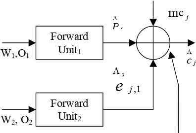
below:Decoder:

Fig 5.4 Decoding phase of the proposed architecture Forward

Unit1

Forward Unit2

W1,O1

W2, O2

j

PΛ

m

c_j

j

cΛ

1 , j

s

e

(40)

CHAPTER 6 IMPLEMENTATION ON THE BOARD

6.1 Overview of the board

The TMS320C6X series of DSP chips are exclusive in that they are the first of their type with

Very Long Instruction Word (VLIW). With VLIW the compiler groups together multiple

instructions that do not have any dependency into a single VLIW instruction. Since the compiler

has done the major task of creating the VLIW instruction stream, the processor now depends on

the compiler to provide it with the VLIW, making it simpler. This has two advantages: the clock

speed increases and the power consumption remains the same. If there are not enough

dependencies between the grouped instructions the compiler pads the VLIW set with NOP

instructions but since image processing and signal processing applications are highly repetitive

numerical computations of large groups of data are not data independent. If the NOP instructions

are padded due to the data dependencies, the processor is not completely utilized so TI came up

with VelociTI technology which reduces the problem of memory usage with VLIW making the

code size smaller. TI also made another improvement with VelociTI.2 which included specialized

instructions for packed data processing for many applications like high – performance and low –

cost image processing [8].

6.2 Floating – Point and Fixed – Point:

In the floating – point architecture the set of real numbers is represented by a single-precision

float data type or a double precision double data type bits for a fraction containing the number of

(41)

Floating point arithmetic is very powerful and is also very convenient in programming except for

the underflow and overflow conditions to be taken care of. If the function of an arithmetic deals

only with the integral values then it is advantageous to use a fixed – point processor as this

processor is faster (clock speed increases) with less power consumption due to the simplicity of

the hardware.

The above proposed algorithm is implemented on the TI DSP TMS320C6713 DSK board in the

floating-point arithmetic. The board is based on high performance, advanced

very-long-instruction-word architecture. This board operates at 225MHz, the C6713 delivers up to 1350

million floating point operations per second (MFLOPS), 1800 million instructions per second

(MIPS) and with dual fixed/ floating point multipliers up to 450 million multiply- accumulate

operations per second (MMACS).

The C6713 uses a two-level cache-based architecture and has a powerful and diverse set of

peripherals. The Level 1 program cache (L1P) is a 4K-Byte direct-mapped cache and the Level 1

data cache (L1D) is a 4K-Byte 2-way set-associative cache. The Level 2 memory/cache (L2)

consists of a 256K-Byte memory space that is shared between program and data space. 64K

Bytes of the 256K Bytes in L2 memory can be configured as mapped memory, cache, or

combinations of the two. The remaining 192K Bytes in L2 serves as mapped SRAM.

The C6713 has a rich peripheral set that includes two Multichannel Audio Serial Ports

(McASPs), two Multichannel Buffered Serial Ports (McBSPs), two Inter-Integrated Circuit (I2C)

buses, one dedicated General-Purpose Input/Output (GPIO) module, two general-purpose timers,

a host-port interface (HPI), and a glueless external memory interface (EMIF) capable of

(42)

The two McASP interface modules each support one transmit and one receive clock zone. Each

of the McASP has eight serial data pins which can be individually allocated to any of the two

zones. The serial port supports time-division multiplexing on each pin from 2 to 32 time slots.

The C6713 has sufficient bandwidth to support all 16 serial data pins transmitting a 192 kHz

stereo signal. Serial data in each zone may be transmitted and received on multiple serial data

pins simultaneously and formatted in a multitude of variations on the Philips Inter-IC Sound

(I2S) format.

In addition, the McASP transmitter may be programmed to output multiple S/PDIF, IEC60958,

AES-3, CP-430 encoded data channels simultaneously, with a single RAM containing the full

implementation of user data and channel status fields.

The McASP also provides extensive error-checking and recovery features, such as the bad clock

detection circuit for each high-frequency master clock which verifies that the master clock is

within a programmed frequency range.

The two I2C ports on the TMS320C6713 allow the DSP to easily control peripheral devices and

communicate with a host processor. In addition, the standard multichannel buffered serial port

(McBSP) may be used to communicate with serial peripheral interface (SPI) mode peripheral

devices.

The TMS320C6713 device has two bootmodes: from the HPI or from external asynchronous

(43)

The TMS320C67x DSP generation is supported by the TI eXpressDSP set of industry benchmark

development tools, including a highly optimizing C/C++ Compiler, the Code Composer Studio

Integrated Development Environment (IDE), JTAG-based emulation and real-time debugging,

and the DSP/BIOS kernel.

6.3 DSP Boards in Image Processing:

In many cases, image processing algorithms are characterized by repetitive performance of the

same operation on a group of pixels. For example, filtering a signal involves repeated

accumulate operations and filtering of an image involves repeatedly performing these

multiply-accumulate operations on each pixel of an image while sliding the mask across the image. These

repeated numerical computations require a high memory bandwidth. All these imply that image

processing involves high computational and data requirements. This can be considered as a

reason why image processing applications are increasingly being done on embedded systems. A

digital image is represented as a matrix but in C/C++ the image matrix is often flattened and

stored as a one-dimensional array. This flattened image can be done in either a row-major or a

column major fashion. In the row major fashion the matrix is stored as an array of rows i.e. all the

elements of a row are first ordered, then the elements of the next row and so on, and is used in

C/C++. In the column major fashion the matrix is stored in the array of columns i.e. all the

elements of a column are ordered first then the elements of the next column and so on, and is

used in MATLAB.In the implementation of image processing applications on any embedded

systems the main problem is inputting the data into the system. The large size input data of an

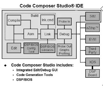
image cannot be directly initialized into an array. Code Composer Studio provides the functions

of basic C like the fwrite, fread, fopen, fclose but these functions are so slow that it is not even

(44)

this CCStudio is built-in with certain input/output facilities like the Real Time Data Exchange

(RTDX) and the High Performance Interface (HPI).

6.4 IMPLEMENTATION OF THE ALGORITHM ON BOARD:

The above proposed algorithm is implemented on this board. The coding part of the algorithm is

done in the Code Composer Studio IDE which is done in the visual studio.

Fig 6.1 Code Composer Studio Architecture from TI Documentation

Code composer studio can be used with a simulator (PC) or can be connected to a real DSP

system and test the software on a real processor board (DSP). In order to write some type of code

on the DSP board a project is to be created, a project consists of source file, library files,

DSP/BIOS configuration, and linker command files. The project has the following settings: Build

(45)

controls many aspects of the build processes such as: optimization level, target device,

compiler/assembly/link options. The step-by-step approach for creating a project with code in the

code composer studio is:

• Open code composer studio.

• Create a project based on C.

• Compile, link, download and debug the program.

• Watch variables

• Break points and probe points can be used

To create projects, go to project on the toolbar, Project->New. Give the project name, select

target type and suitable location of the hard disk. The project creates a subdirectory by itself in

the location specified.

To write the source codes, go to file on the toolbar, File->New->Source file. Save the file as *.C

(46)

The C source code is now stored in the project subdirectory of the hard disk but it is not a part of

the project yet. So, to add it to the project: Project->Add files to the project, browse to the

location of the source code and say OK.

Compile the source code by, Project->Compile File. The active source code (the code of the

project) will be compiled and if there are any errors they are displayed.

To run the source code the source code is to be linked. Linking is done by adding certain linker

library files provided by the TI. This can be done by Project->Build options->Linker->Library

search path (c:\ti\c2000\cgtools\lib) and Project->Build Options->Linker->include libraries

(c:\ti\c2000\cgtools\rts2000_lib).

(47)

The linker puts together the various building blocks needed for the system. This is done with

“Linker Command File”. This is used to connect the physical memory parts of the DSP’s

memory with the logical sections of the system. Add the linker command file by: Project->Add

files to the project. A command file can be written by the user according o his needs. Then Build

the project: Project->Build.

Linking connects one or more object files (*.obj) into an output file (*.out). This file not only

(48)

Now to load the code onto the DSP: File->Load program->Debug\*.out. To run the code:

Debug->run.

DSP/BIOS:

DSP/BIOS tool for the Code Composer Studio software is designed to minimize memory and

CPU requirements on the target. This can be done by:

• All DSP/BIOS objects can be created in the configuration tool and put into the main

program image. This reduces the code size and even optimizes the internal data structures.

• Communication between the target and the DSP/BIOS is performed within the

background idle loop such that the DSP/BIOS do not interfere with the main program.

• Logs and Traces used to output, input or for the timed processes are formatted by the host.

• A program can dynamically create and delete objects to be used in the special situations.

• Two I/O models are supported for maximum flexibility and power. Pipes are used for

target/host communication and to support simple I/O cases where a thread writes to the

pipe and another thread reads from the pipe. Streams are used for more complex I/O

operations.

DSP/BIOS is a real time kernel designed for the applications that require scheduling and

synchronization, host – to – target communication or real – time instrumentation.

Optimizing C/C++ Code:

A C/C++ program performance can be maximized by using the compiler options, intrinsics and

code transformations such as software pipelining and loop unrolling. The compiler has three

basic stages when compiling any loop: qualify the loop for software pipelining, collect loop

(49)

the compiler options make a code fully optimized. The C6x compiler provides intrinsics,

functions designed specially to map to the inlined instructions to optimize the code quickly.

Intrinsics are specified with an underscore ( _ ) in front of them and are called as any other

function is called. For example in the implementation of this thesis there are a few intrinsics used

like: _amemd8 , this is equivalent to the assembly operations Load word/Store word allows

aligned loads and stores of 8 bytes to memory and can be used on all the C6x boards. _extu is

equivalent to extract in the assembly and is used to extract a specified field in src2, sign extended

to 32 bits. The extract is performed by a shift left followed by a unsigned shift right. _itod is

used to create a double register pair from two unsigned integers. _hi, returns the high 32 bits of a

double as an integer. _lo returns the low register of a double register pair as an integer. There are

a more of the intrinsics available and can be seen in the TI documentation.

This thesis is put into the DSP processor in the following way: A project compress.pjt is created

as said above. Then a C source file compress.c is written. This file contains all the necessary

coding for the proposed algorithm. The main part in this implementation is the memory

allocation, image loading and memory management. As a large amount of memory is required all

the memory allocations and freeing of memory for not so much necessary variables are first done.

Then the source file is added to the project. All the necessary library files are also added to the

project. The include files are checked to be seen in the project. Then in the DSP/BIOS the

memory is assigned. In the DSP/BIOS the system is enlarged and in it the SDRAM is selected. In

order to change the size of memory the properties of the SDRAM needs to be checked. In the

properties dialog box the starting address, stack size and the heap size are given. Heap is the

actual memory we are using out of the stack and hence the heap is always to be smaller than the

stack size. The image dimensions of this thesis are taken as 512x512. Due to the size of the

(50)

pragma (compiler directive) tells the CCStudio to allocate space for the symbols as SDRAM in

this case for the input image, image1. So for the linker command file to know this the memory

segment in the DSP/BIOS is configured appropriately. A matlab code is written to convert the

image into an ASCII text file. This text file is used by the CCS to import data into the DSP. The

text file is generated such that each line contains a single word of data. After building the project

and loading the executable program onto the DSP, a breakpoint is set in main where the image

load is printed. When the program is run the debugger stops at this line. By using the

FILE->DATA->LOAD menu item the block of image data is sent into the DSP. When the LOAD

dialog box comes up the address where the text file is stored is given, then in the format “Hex” is

chosen. By clicking ok on this dialog box the next dialog box allows the user to specify the

memory location where it is to be saved, asking for the destination and the data length which in

this case is taken as 65536. In order to view the image at any point in the code

VIEW->GRAPHS->IMAGE then in the dialog box enter the memory point (variable) to be viewed and

the size of the variable(image). To view the contents of any memory location

VIEW->MEMORY. The image in the present code then is divided into the blocks then the mean,

estimation, encoding and decoding are done as per the algorithm specified in the previous

Hardware Implementation of a Novel Image Compression Algorithm

ScholarWorks@UNO

ScholarWorks@UNO

Hardware Implementation of a Novel Image Compression

Hardware Implementation of a Novel Image Compression

Algorithm

Algorithm

HARDWARE IMPLEMENTATION OF A NOVEL IMAGE

COMPRESSION ALGORITHM

ACKNOWLEDGEMENTS

TABLE OF CONTENTS

LIST OF TABLES

LIST OF FIGURES

ABSTRACT

CHAPTER 1

INTRODUCTION

CHAPTER 2

TECHNIQUES OF IMAGE COMPRESSION

CHAPTER 3

IMAGE COMPRESSION USING JPEG STANDARD

[

] [ ] [ ]

[

]

(

)

(

)













Π

+













Π

+

=

∑

∑

2

1

2

cos

2

1

2

cos

,

,

N

k

n

N

k

n

n

n

x

k

c

k

c

k

k

X

[

]

[

] [

]

(

)

_

_