Volume 4 - Article 9 | Pages 289–336

in the population sciences published by the Max Planck Institute for Demographic Research Doberaner Strasse 114 · D-18057 Rostock · GERMANY www.demographic-research.org

DEMOGRAPHIC RESEARCH

VOLUME 4, ARTICLE 9, PAGES 289-336

PUBLISHED 12 JUNE 2001

www.demographic-research.org/Volumes/Vol4/9/

DOI: 10.4054/DemRes.2001.4.9

Application of the Demographic Potential

Concept to Understanding the Russian

Population History and Prospects:

1897-2100

Dalkhat Ediev

1. Introduction 290 1.1 What to be examined and how 290 1.2 Concept of demographic potential and its

application to population analysis

291

2. Data 293

3. Population and demographic potential trends since 1897

294

3.1 General perspective 294

3.2 Different stages of Russian population history 299 3.2.1 Russian population dynamic before World War I 299 3.2.2 Russian population after World War I and before

the mid 1920s

299

3.2.3 Russia between the Civil War and World War II (1923-1941)

299

3.2.4 Consequences of World War II and postwar trends in Soviet Russia

300

3.2.5 Russian population after the crush of the Soviet Union

302

4. Demographic prospects of Russia 302 4.1 Results and implications of US Census Bureau

projections

302

4.2 Alternative scenarios of Russian population trends in the XXI century

303

4.3 Can fertility recovery or higher immigration keep Russia from depopulation?

306

4.4 Comparative analyses of different population projections

309

5. Conclusions 311

6. Acknowledgements 311

Notes 312

References 312

A. Appendix A. Concept of demographic potential and related issues

319

A.1 Fishers’ reproductive value 319 A.2 Potential of population growth 321 A.3 Stable equivalent and population momentum 322

A.4 Demographic potential 325

B. Appendix B. Aggregate population modeling and forecasting

Application of the Demographic Potential Concept to Understanding

the Russian Population History and Prospects

1897-2100

Dalkhat Ediev 1

Abstract

The article deals with Russian population estimates since 1897 and prospects to the end of the XXI century. Concept of demographic potential is used to examine past trends and project future tendencies. Dramatic disturbances of the past century hampered population growth and brought the possibility of halving the Russian population, the possibility, which could turn into inevitability if demographic problems are not solved before the mid-XXI. At the same time the Russian population still has a momentum of quick growth under the condition of fast recovery of vital rates.

1 _{Karachay-Cherkessian State Technological Institute, Department of Highest Mathematics and}

1. Introduction

1.1 What to be examined and how

Entering the XX century as one of the largest countries of the world, having high fertility, huge land area, and abundant resources, Russia had perspectives for economic growth, life expectancy improvements and many-fold population increase. Nonetheless Russian population only doubled in the XX century and this growth happened mostly due to the age structure changes. Why was Russian population growth so slow in the last century? What could happen to the population in the future? How fast should the fertility recovery be in order to overcome present demographic problems of Russia? Can immigration help in avoiding the depopulation of Russia? Using the demographic potential approach (Ediev 1999, 2000, 2001), these questions are addressed in this paper taking into consideration the long-range population dynamics of Russia (1897-2100).

Despite relatively scarce data, a great number of works exploring Russian (Soviet Union in its time) population trends and perspectives are available both in Russia (e.g. Center for Demography and Human’s Ecology 2000, 2001, Goskomstat Rossii 1998, Andreev, Darsky, and Khar'kova 1993, 1998, Vishnevsky and Volkov 1983, Sifman 1974, let alone statistical and analytical yearbooks) and in the West (Blum and Avdeev 2000, U.S. Bureau of the Census 1980, 1997, 2000, United Nations 1992, 1999, Hollander 1997, Shkolnikov, Mesle, and Vallin 1996, DaVanzo and Farnsworth 1996, Chen, Wittgenstein, and McKeon 1996, Barkalov and Darsky 1994, Keyfitz and Flieger 1990, Anderson and Silver 1989, Pressat 1985, Berent 1970a, 1970b). Researchers pay special attention to Russian population losses caused by wars, revolution, repression, deportations, and famine (Andreev, Darsky, and Khar'kova 1990, 1993, and 1998, Wheatcraft 1981, 1990, and 1995, Denisenko and Shelestov 1994, Livi-Bacci 1993, Polyakov 1986, Maksudov 1989, Anderson and Silver 1985, Davies and Wheatcroft 1984, Rosefielde 1983, 1984, Dyadkin 1983, Boyarsky 1975, Urlanis 1968, Eason 1959, Timasheff 1948, Lorimer 1946).

projection scenario called “no disturbances”. Latter scenario examines last century’s population trends, which could take place in the absence of such cataclysms as wars, famine, etc. Different projection scenarios are examined to explore the future of Russian population as well. An aggregate population model is used to get forecasts of the Russian population, the model based on the demographic potentials concept.

1.2 Concept of demographic potential and its application to population analysis

Following is a brief description of the demographic potential concept and its applications to population studies. More detailed discussion of the demographic potential concept, its application to population modeling, and a review of related works are presented in Appendixes A and B.

Demographic potential is an aggregate index related to ultimate posterity of the population. It reflects the demographic power of the nation, its ability to provide future population growth. Future perspectives depend on a wide variety of factors, mostly unpredictable. That’s why the purpose of demographic potential is not to measure

actual population perspectives. Rather, demographic potential is aimed to reflect the current weight of the population, its potential ability to grow under appropriate external conditions. For one-sex stable population it turns into R. A. Fisher’s (Fisher 1930) reproductive value (see Appendix A). Given the potentials for different age groups and age structure of the population, aggregate demographic potential can be calculated as:

( )

=

_∫

∞

( ) ( )

0

;

t

c

x

dx

x

n

t

C

, (1)

here C(t) is total demographic potential, c(x) is the demographic potential of the average

person aged x, and

n

( )

x

;

t

is population density at exact age x at time t. Although the potential (1) relates to one-sex population, a two-sex generalization can be developed,

which is used in this work:

( )

t

(

1

γ

)

C

( )

t

C

( )

t

/

γ

C

total

=

+

female

⋅

male (2)

here

C

_population

( )

t

is the aggregate demographic potential of given population at time t;

γ

is the sex ratio at birth (males to females).

by changes in age-sex composition. To be accurate, this property holds only for a stable population with demographic potentials based on its own reproduction parameters. Yet, the author's experience shows that even for real populations the change rate of demographic potential is a good approximation for intrinsic growth rate. The situation is different when the population size is considered. Population is heavily affected both by the intrinsic growth and by changes in the age composition. Therefore, its change rate can’t be used to make conclusions about the mechanics of the population growth. Population can grow due to high fertility or aging - depending on phase of demographic transition. Migration can also play a significant role in the dynamic of demographic potential in addition to the intrinsic growth. Therefore, demographic potential’s growth can be attributed mainly to the role of over-replacement fertility and immigration, while the population is additionally affected to the changes in population composition.

This observation is helpful in decomposing the population change rate into rates imposed by intrinsic growth and the age structure changes. If, for example, the population increased by 25%, but demographic potential remained constant, then the growth happened mostly due to the age structure changes alone. If in the same situation demographic potential grew by 10%, then only this increase was “real” (generally speaking it happened due to the excess of fertility over the replacement level and due to the immigration), while the rest can be attributed to the age structure changes (1.25/1.10=1.14, i.e., 14%) and a combination of both factors (25-10-14=1%). The interpretation that only changes in demographic potential are real is justified by the fact that it is the total demographic potential, which mostly determines the asymptote of the population. Two populations having the same demographic potentials and the same reproduction regime in future will ultimately have the same size despite any differences in their age-sex composition at the beginning. Demographic potential decline results in ultimate depopulation and its growth leads to a population increase. The decomposition mentioned above is fulfilled in the paper to explore, whether the population changes were caused by the fertility above the bare replacement, or they were caused by the age structure adjustments.

Some comments are to be made about the role of the mortality and fertility in dynamic of the demographic potential. Being the only real solution of the equation

( ) ( )

∫

∞

−

=

0

1

l

y

f

y

e

ρy

dy

,

(3)

the intrinsic rate of natural increase

ρ

apparently depends both on the fertility and the

of one. Hence the deviations of the intrinsic growth rate from its trend usually reflect changes in the fertility rather than in the mortality level. There are two main exceptions to this rule. Firstly, at the beginning of the demographic transition intrinsic growth rate can increase due to decrease in mortality at childbearing ages and below. This was the case of Russia in 1940s, when at the end of the World War II infant mortality in Russia decreased by almost 50% due to use of advanced medicines (Sifman 1979). Secondly, unusual mortality changes, which accompany wars, famine, etc. highly affect the intrinsic growth rate and the demographic potential. These events aren’t examined in terms of intrinsic rates however. Rather, they are examined in terms of population and potential losses.

2. Data

Data on age-sex composition of the population are primarily used in the paper. Data were taken from different sources. The long-range data set is provided in a publication of the Russian Statistical Agency (Goskomstat Rossii 1998). Data for Stalin’s period were reconstructed by a team of Russian demographers (Andreev, Darsky, and Khar'kova 1998). For the period after 1960 population data were published in Russian and Soviet statistical yearbooks. In addition to sources described above some useful data were obtained from International Data Base of the US Census Bureau (U.S. Bureau of the Census 1999), which provides projections of population age-sex structure as well as historical data (available for Russia since 1989).

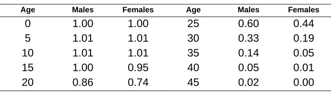
Demographic potentials used in the paper (Table 1) are based on US 1991 data (National Center for Health Statistics 1995, University of California, Berkeley 1998). It has been made both for the sake of comparability with results obtained earlier and in order to make use of aggregate population models based on demographic potentials pattern mentioned (Ediev 2000, 2001).

Table 1: Age-sex specific demographic potentials (5-year age intervals). US 1991.

Age Males Females Age Males Females

0

1.00

1.00

25

0.60

0.44

5

1.01

1.01

30

0.33

0.19

10

1.01

1.01

35

0.14

0.05

15

1.00

0.95

40

0.05

0.01

3. Population and demographic potential trends since 1897

3.1 General perspective

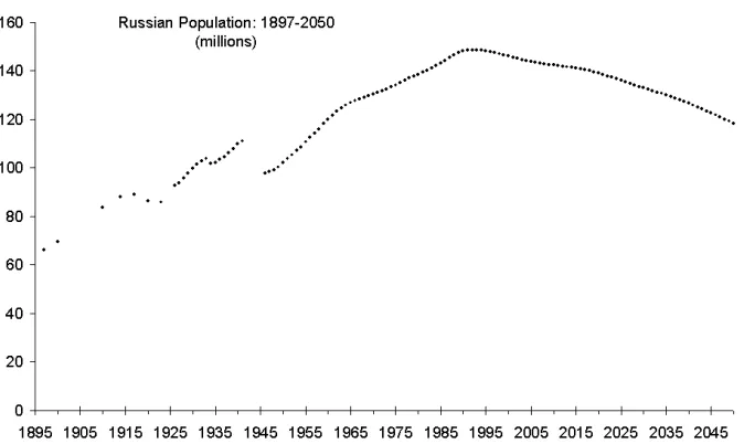
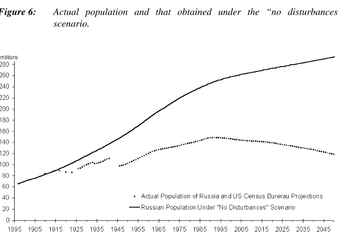
Russian population trends since 1897 as well as a projection until 2050 (U.S. Bureau of the Census 2000) are presented in Fig. 1. Despite two World Wars, the Revolution of 1917, the Russian Civil War, famine in 20s and 30s, and recent socioeconomic problems, the population in Russia has grown in the XX century. It happened due to two main factors – intrinsic growth (i.e., high fertility) and the age structure changes, as it usually happens in the process of demographic transition. Roles of these two forces – intrinsic growth and the age structure changes – can be separated comparing the population trend (Fig. 1) to that of demographic potential (Fig. 2).

Figure 1: Russian population in 1897-2050 (millions).

migration), 48% – due to the age structure changes (caused by life expectancy improvements and young age structure of initial population), and 19% – due to interaction of both factors.

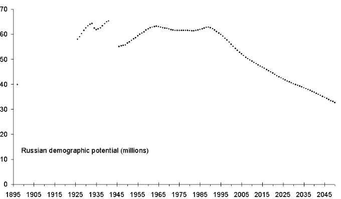
Figure 2: Russian demographic potential in 1897-2050 (millions).

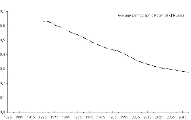
accurate relation). Hence Fig. 3 reflects the dynamic of Vincent’s potential of Russia, i.e., of its momentum as well.

Figure 3: Average Russian’s demographic potential. 1897-2050.

Figure 4: Demographic potential’s change rate: actual and that used in the “no disturbances” scenario.

Figure 5: Russian demographic trends under the “no disturbances” scenario.

Figure 6: Actual population and that obtained under the “no disturbances”

3.2 Different stages of Russian population history

Following the trends of population and demographic potential, several demographic stages in Russian population history can be pointed out:

after 1897 and before World War I; after World War I and till the mid-1920s; after end of the Civil War and till World War II; after World War II and till the 1960s;

the 1960s to the 1980s;

the reform and post-reform period.

3.2.1 Russian population dynamic before World War I

In spite of defeat in the Russian-Japanese War and the Revolution of 1905, Russia grew without significant deviations from the “no disturbances scenario” between 1897 and 1914. This period was characterized by high mortality and high fertility as well. TFR at the level of 5-7 implied demographic potential’s growth rate of more than 2% yearly despite life expectancy at birth of about 30 years and remarkable emigration from the country.

3.2.2 Russian population after World War I and before the mid 1920s

World War I followed by the Revolution, the Civil War, high emigration, intervention, and famine of 1921-1922 depressed the Russian population trend dramatically (Fig. 6). The “no disturbances” scenario leads to the population of 103 mln. in 1923, while the actual figure was only 86 mln., i.e., about 17 mln. of the possible population in 1923 or about half of all the possible population growth since 1897 was lost.

3.2.3 Russia between the Civil War and World War II (1923-1941)

lowered fertility afterwards. As early as 1934 the population increased, but this happened due to the age structure changes rather than fertility recovery – the demographic potential increased only a year later (Fig. 3). Relatively fast growth of the demographic potential started only in 1937/38; it happened partly as compensation and partly as a result of the abortions prohibition in 1936. The growth was slowing down and later World War II interrupted it. Under the “no disturbances” scenario mentioned above, the population grows 108% by 1941, while actual growth was only 68%. I.e., almost half (37%) or 26 mln. of possible population growth was lost due to dramatic events at the beginning of the century. This estimate is consistent with other estimates of Russian demographic losses before the 1940s (Denisenko and Shelestov 1994, Andreev, Darsky, and Khar'kova 1993, Wheatcraft 1990, Maksudov 1989, Anderson and Silver 1985, Boyarsky 1975, Lorimer 1946).

Figure 7: Male/female ratio of demographic potentials in Russia.

3.2.4 Consequences of World War II and postwar trends in Soviet Russia

Male potential was more affected by the War than that of females; its loss was at the level of 20% while female’s potential loss was about 12%. This selective effect increased gender disparity (Fig. 7), which determined social problems in decades to come. These losses weren’t the only consequences of the War. It affected the fertility trend as well. After World War II potential grew much more slowly than before, while it should have grown faster under the compensation baby boom. Postwar growth of demographic potential was modest (0.76% annually between 1946 and 1963) and insufficient to make up for wartime losses. This is even more remarkable if we take into account the fact of unprecedented decrease in child mortality during wartime (Zakharov 1996, Sifman 1979) and later life expectancy improvements (Andreev, Darsky, and Khar'kova 1998). The famine of 1947, which cost the Russia about half a million lives (Andreev, Darsky, and Khar'kova 1998) was one of the low fertility causes in late-40s. In addition to the low fertility the postwar change in sign of migration flows wasn’t in favor of Russia. The Russian population had negative migration balance after World War II and till the mid-70s.

In the 1960s the new actor – the process of urbanization – played its dramatic role. While before World War II Russia was a rural country, as early as at the beginning of the 1960s its population was living primarily in urban areas. Rural population had high fertility, but it moved to urban areas with low fertility that brought the country to a level of replacement: since the 1960s fertility dropped and demographic potential became almost constant till the end of the USSR. Life expectancy was already stagnating at that time as well (Goskomstat Rossii 1998). The fact that the population continued to grow at that period reflects the impact of the age structure momentum accumulated before. The slight growth of the demographic potential in the 1980s was due to the Soviet government's attempts to encourage fertility and a positive shift in external migration.

Figure 8: Dynamic of Russian female demographic potential (millions) – actual and hypothetical, at zero migration at reproductive ages, 1979-1996.

3.2.5 Russian population after the crush of the Soviet Union

The last stage begins with Gorbachev’s perestroika, the collapse of the USSR, and following reforms (consequences of Chechenian conflict aren’t counted here due to lack of data). Fertility dropped dramatically and as a result Russian demographic potential declined in 1989-2000 with annual rate of about 1% and became 14% less in 2000 than before World War II despite tangible immigration to the country. At the same time mortality grew till the mid-90s and then slowed down again. Recent results (Shkolnikov and Vishnevsky 2000) show, however, that the 1990’s mortality growth was probably a compensational growth after the decline in the late 1980s (due to the anti-alcohol campaign), rather than a “cost of reforms”. Anyway, the fertility decline caused by the last socio-political and economic transition resulted in an unprecedented decrease of demographic potential and opened the way to the deep depopulation of Russia.

4. Demographic prospects of Russia

4.1 Results and implications of US Census Bureau projections

50% (life expectancy improvements could lower this estimation to about 40%). Although the Russian population will be only 20% less in 2050 compared to 1989, it will be much more aged at that time (Fig. 9), which will further accelerate the population decline.

Figure 9: Age-sex composition of Russia according the US Census Bureau

projection.

Is it possible to escape from this depopulation trap? How could it be possible is put to question below by examining different population projection scenarios.

4.2 Alternative scenarios of Russian population trends in the XXI century

The Center for Demography and Human’s Ecology made Russian population projections up to 2020 using component methods and a multiregional approach (Andreev and Khar'kova 2000). Assumptions of these forecasts as well as additional assumptions about the dynamics after 2020 are used in this paper to get “low”, “medium”, and “high” variants. The following standard procedures are used to get assumptions after 2020. All the parameters driving the population projection in demographic potential projection technique – life expectancy at birth, intrinsic growth rate, and immigration – are set to be constant after 2050 (life expectancy being 80; intrinsic growth at the replacement level, i.e., 0%; and immigration at the level of zero). These parameters are interpolated linearly between 2020 and 2050.

Now let us proceed with a discussion of projections results.

In the “low” scenario the intrinsic growth rate starts from about –3% in 2020 (TFR of 1.01) and increases up to the replacement level in 2050. Results of projection within this scenario are presented in Fig. 10. In 1989-2050 the population declines by 47%. In the same period demographic potential declines by 69%, predetermining further depopulation. As a result, by the end of the next century the population will have declined by 62% with respect to 1989 (discrepancy between last two figures can be attributed to the role of life expectancy improvements). In this scenario the Russian population ultimately stabilizes at the level of 38% of current population, i.e., 56 mln.

Figure 10: Russian population projection within the “low” scenario.

In the “high” variant the population decreases by 24% in 2050 and by 37% in 2100 with respect to 1989 (Fig. 12). Demographic potential decreases by 48%. Ultimately the Russian population stabilizes at 64% of the current level, i.e., depopulation stops at 93 mln.

Figure 12: Russian population projection within the “high” scenario.

4.3 Can fertility recovery or higher immigration keep Russia from depopulation?

The next scenarios aren’t just a transition from variants of the Center for Demography and Human’s Ecology to the stationary model. These projections are made in order to examine if different demographic improvements can prevent the Russia from deep depopulation. These models are based on the “high” variant’s assumptions with different corrections depending on the scenario.

forecasts, and high immigration at the beginning combined with fertility improvements lead to a steady population increase and a stationary level of about 170 mln. This is 16% more than the current population. Demographic potential under fast recovery becomes 3% less in 2100 compared to 1989, but 8% more than in 2000.

Another scenario, “late recovery”, assumes that the baby boom will happen only after 2050 (Fig. 14). As mentioned above, the Russian population will be very aged in 2050, and will not be as sensitive to fertility recovering after that. Under this scenario the population never grows in the XXI century, decreases by 28% in 2100 with respect to the current population, and stabilizes at the level of 106 mln. Only life expectancy growth up to 80 years prevents the population decrease by about 40% in this scenario following the same loss of demographic potential. As a result, Russian 2100 population under fast recovery is about 60% higher than that under the late recovery.

Figure 14: “Late recovery” scenario.

The last scenario (“high immigration”, Fig. 15) addresses the possibility of compensating for low fertility with a higher immigration rate. In this scenario everything is the same as in “high” scenario plus an additional immigration flow of 0.5% in 2010-2040 (by the year 2050 population returns to the stationary pattern as in scenarios above). Resultant immigration in 2010 is about three-fold higher than in the “high” scenario. At the beginning of the XXI century such a substantial additional immigration leads to population growth. Yet, immigration can’t compensate for low fertility in the long term. Demographic potential declines and finally population size decreases too. As a result, by 2100 the population decreases by 21% and demographic potential decreases by 35% with respect to 1989. Finally, the population stabilizes at the level of 116 mln. (79% of current population).

4.4 Comparative analyses of different population projections

Figs. 16 and 17 summarize population projection results under all the scenarios mentioned with two additions. First, the result of projection under the “no disturbances” scenario mentioned above is added to the figure in order to compare past trends and future scenarios to what the Russian population would be were it not for the socio-political problems of last century. Secondly, the US Census Bureau’s projection is prolonged till 2100 under zero migration, 80-year life expectancy, and replacement fertility assumptions (like in all other projections).

Figure 16: Russian population: past trends and future projections under different assumptions (1897-2100).

Figure 17: Russian demographic potential: past trends and future projections under

It can be seen (Fig. 16) that almost all the future scenarios (except for “fast recovery”) lead to remarkable depopulation of Russia. Even high immigration or late recovery of vital rates can not help. Up to 40-60% of the current population can be lost if this depopulation happens. It means that Russia would loose up to 70-80% of its possible population compared to the “no disturbances” scenario due to the historical cataclysms of the XX century and their consequences. Fast fertility recovery provides better results than the “high immigration” scenario in the nearest future and leads to steady population growth in the long-range as well, restoring the pre-reform population status quo.

5. Conclusions

Russian population growth in the XX century was interrupted and hampered by dramatic events: wars, revolution, emigration, famine, urbanization, and socioeconomic transition. These events have already cost Russia about a half of its possible population in 2000. If reproductive patterns in Russia remain on a low level till the mid-XXI century, the country could face further population halving and even deeper decline. At the same time, fast fertility recovering can instantly result in steady population growth up to about 170 million. But if demographic improvements are delayed till the mid-century, the population will be very aged and deep depopulation will be almost inevitable. Immigration could partly compensate for the effect of low fertility and delay the process of depopulation; but it should be at the level of at least 0.5-1% annually.

6. Acknowledgements

Notes

An Excel spreadsheet with the aggregate population projecting model used in this paper can be downloaded from the Demographic Research web site. Please see the introductory HTML cover sheet for this paper at http://www.demographic-research.org/volumes/vol4/9/ .

References

Anderson B. A., Silver B. D. (1985). “Demographic analysis and population catastrophes in the USSR”. Slavic Review, 44, 3: 530-531.

Anderson, B. A., Silver, B. D. (1989). “Demographic Sources of the Changing Ethnic Composition of the Soviet Union”. Population and Development Review, 15: 609-656.

Andreev, E. M., Darsky, L. E., Khar'kova, T. L. (1990). “Estimation of Population Losses During the Great Patriotic War of 1941-1945 Using the Method of Demographic Balance” (in Russian). Vestnik statistiki, 9: 25-27.

Andreev, E. M., Darsky, L. E., Khar'kova, T. L. (1993). Population of the Soviet Union: 1922-1991 (in Russian). Moscow: Nauka.

Andreev, E. M., Darsky, L. E., Khar'kova, T. L. (1998). Demographic history of the Russia: 1927-1959 (in Russian). Moscow: Informatika.

Andreev, E. M., Khar'kova, T. L. (2000). Russian Population Forecast to 2020. In: Center for Demography and Human’s Ecology. Population of Russia 1999. 7th annual report (in Russian). Ed. Vishnevsky A.G. Moscow: Knizhny Dom «Universitet»: 156-164.

Andreev, E. M., Pirozhkov, S. I. (1975). On the potential of demographic growth. In: Naselenie I Okruzhajushaja Sreda. Moscow.

Arthur, W. B. (1982). “The Ergodic Theorems of Demography: a Simple Proof.”

Demography, 19: 439-445.

Barkalov, N. B., Darsky, L. E. (1994). Russia: Fertility, Contraception, Induced Abortion, and Maternal Mortality. The Futures Group.

Berent, J. (1970b). “Causes of Fertility Decline in Eastern Europe and the Soviet Union II: Economic and Social Factors”. Population Studies, 24: 247-292.

Blum, A., Avdeev, A. (2000). Demography of Russia and Empire (in French). http://www-census.ined.fr/demogrus/

Bourgeois-Pichat, J. E. (1968). The Concept of a Stable Population. Application to the Study of Populations of Countries With Incomplete Demographic Statistics. N.Y.: United Nations.

Bourgeois-Pichat, J. E. (1971). “Stable, Semi-stable Populations and Growth Potential”.

Population Studies, 25: 235-254.

Boyarsky A. J. (1975). Population and methods of population analysis (in Russian). Moscow: Statistica.

Center for Demography and Human’s Ecology. (2000). Population of Russia 1999. 7th annual report (in Russian). Ed. Vishnevsky A.G. Moscow: Knizhny Dom «Universitet», 2000.

Center for Demography and Human’s Ecology. (2001). Demoscope Weekly. Electronic version of the Population and Society (in Russian). http://demoscope.ru/

Cerone, P. (1996). “On the effects of the generalized renewal integral equation model of population dynamics”. Genus, 52: 53-70.

Chen, L. C., Wittgenstein, F., McKeon, E. (1996). “The Upsurge of Mortality in Russia: Causes and Policy Implications”. Population and Development Review, 22: 517-530.

Cole, L. C. (1965). Dynamics of animal population growth. In: M. C. Sheps and J. C. Ridley (eds.), Public Health and Population Change: Current Research Issues. Pittsburgh: University of Pittsburgh Press.

DaVanzo, J. S., Farnsworth, G. (1996). Russia's Demographic "Crisis". RAND doc no. CF-124-CRES. http://www.rand.org/publications/CF/CF124/

Davies, R. W., Wheatcroft, S. G. (1984). “A Note On Steven Rosefielde’s Calculations of Excess Mortality in the USSR. 1929-1949”. Soviet Studies, 36: 277-281. Denisenko M. B., Shelestov D. K. (1994). Population losses. In: Melikyan G. G.,

Kvasha A. J., Tkachenko A. A., Shapovalova N. N., Shelestov D. K. Population (in Russian). Moscow: Big Russian Encyclopedia: 342-345.

Eason, W. W. (1959). “The Soviet Population Today”. Foreign Affairs, 37: 601. Ediev, D. M. (1999). Demographic and economic-demographic potentials (in Russian).

Ph.D. thesis. Moscow: Moscow Institute of Physics and Technology.

Ediev, D. M. (2000). “Principles of Aggregate Demographic-Economic Modeling Based on Demographic Potentials’ Technique”. Presentation to the workshop on Demographic-Macroeconomic Modeling (Oct. 11-13, 2000). Rostock: Max Plank Institute for Demographic Research. http://www.demogr.mpg.de/Papers/workshops/ws001011.htm

Ediev, D. M. (2001). "Aggregate Population Forecasting With the Use of Demographic Potentials Technique". Investigated In Russia, 38e: 408-431. http://zhurnal.ape.relarn.ru/articles/2001/038e.pdf

Espenshade, T. J. Campbell, G. (1977). “The Stable Equivalent Population, Age Composition, and Fisher’s Reproductive Value Function”. Demography, 14: 77-86.

Fisher, R. A. (1930). The genetical theory of natural selection. N.-Y.: Dover Publications.

Frauenthal, J. C. (1975). “Birth Trajectory Under Changing Fertility Conditions”.

Demography, 12: 447-454.

Frejka, T. (1968). “Reflections on the Demographic Conditions Needed to Establish a U.S. Stationary Population Growth”. Population Studies, 22: 379-397.

Frejka, T. (1973). The Future of Population Growth. N. Y.: John Wiley & Sons.

Goodman, L. A. (1953). “Population Growth of the Sexes”. Biometrics, 9: 212-225. Goodman, L. A. (1967a). “On the Age-Sex Composition of the Population That Would

Result From Given Fertility and Mortality Conditions”. Demography, 4: 423-441.

Goodman, L. A. (1967b). “On the Reconciliation of Mathematical Theories of Population Growth”. Journal of the Royal Statistical Society, Ser. A (General), CXXX: 541-553.

Goodman, L. A. (1968). “An Elementary Approach to the Population Projection-Matrix, to the Population Reproductive Value, and to Related Topics in the Mathematical Theory of Population Growth”. Demography, 5: 382-409.

Hersch, L. (1944). De la demographie actuelle a la demographie potentielle. Gen.

Hollander, D. (1997). “In Post-Soviet Russia, Fertility Is on the Decline; Marriage and Childbearing are Occurring Earlier”. Family Planning Perspectives, 29: 92-94. Kendall, D. G. (1949). “Stochastic Processes and Population Growth”. Journal of Royal

Statistical Society, B, 11: 230-264.

Keyfitz, N. (1968). Introduction to the Mathematics of the Population. Reading, Mass.: Addison-Wesley.

Keyfitz, N. (1969). “Age Distribution and Stable Equivalent”. Demography, 6: 261-269.

Keyfitz, N. (1971). “On the momentum of Population Growth”. Demography, 8: 71-80. Keyfitz, N. (1985). Applied mathematical demography. N. Y., etc.: Springer.

Keyfitz, N., Flieger, W. (1968). World Population: An Analysis of Vital Data. Chicago: The University of Chicago Press.

Keyfitz, N., Flieger, W. (1990). World Population Growth and Aging: Demographic Trends in the Late Twentieth Century. Chicago and London: The University of Chicago Press.

Kim, Y. J. Schoen R. (1997). “Population momentum expresses population aging”.

Demography, 34: 421-427.

Kim, Y. J. Schoen R. Sarma, P. S. (1991). “Momentum and the growth-free segment of a population”. Demography, 28: 159-173.

Leslie, P. H. (1948). “Some Further Notes on the Use of Matrices in Population Mathematics”. Biometrika, XXXV: 213-245.

Livi-Bacci, M. (1993). “On the Human Costs of Collectivization in the Soviet Union”.

Population and Development Review, 19: 743-766.

Lorimer F. (1946). The population of the Soviet Union: history and prospects. Geneva: League of Nations.

Lotka, A. J. (1922). “The stability of the normal age distribution”. Proceedings of the National Academy of Sciences (USA), 8: 339-345.

Maksudov, S. (1989). Demographic losses of the population of the USSR. Benson (Vermont): Chalidze Publications.

Mitra, S. (1976). “Influence of instantaneous fertility decline to replacement level on population growth: an alternative model”. Demography, 13: 513-519.

Mitra, S. (1987). “Models of birth trajectories with certain patterns of variation in vital rates”. Genus, 43: 1-14.

National Center for Health Statistics (USA). (1995). Vital statistics of the United States, 1991. Vol. I. Natality. Washington: Public Health Service.

Polyakov, U. A. (1986). Soviet Country After the Civil War: Territory and The Population (in Russian). Moscow.

Potter, R. G. Wolowyna, O. Kulkarni, P. M. (1977). “Population Momentum: A Wider Definition”. Population Studies, 31: 555-569.

Pressat, R. (1985). “Historical Perspectives on the Population of the Soviet Union (in Data and Perspectives)”. Population and Development Review, 11: 315-334. Preston, S. H. (1986). “The relation between actual and intrinsic growth rates”.

Population Studies, 40: 343-351.

Preston, S. H. Coale, A. J. (1982). “Age structure growth, attrition, and accession: a new synthesis”. Population Index, 48: 215-259.

Rosefielde, S. (1983). “Excess Mortality in the Soviet Union: A Reconsideration of the Demographic Consequences of Forced Industrialization, 1929-1949”. Soviet Studies, 35: 385-409.

Rosefielde, S. (1984). “Excess Collectivization Deaths, 1929-1933. New Demographic Evidence”. Slavic Review, 43, 1: 83-88.

Schoen R., Kim, Y.J. (1991). “Movement toward stability as a fundamental principle of population dynamics”. Demography, 28: 455-466.

Shkolnikov, V. M., Vishnevsky A.G. (2000). Mortality and Life Expectancy. In: Center for Demography and Human’s Ecology. Population of Russia 1999. 7th annual report (in Russian). Ed. Vishnevsky A.G. Moscow: Knizhny Dom «Universitet»: 103-118.

Sifman, R. I. (1974). Dynamic of the Fertility In the USSR (in Russian). Moscow: Statistika.

Sifman, R. I. (1979). On the Causes of Infant mortality Decrease During the Great Patriotic War. In: Life Expectancy: Analysis and Modeling (in Russian). Moscow: Statistika: 50-60.

Timasheff, N. S. (1948). “The Postwar Population of the Soviet Union”. The American Journal of Sociology, 54, 2: 155.

Tognetti, K. (1976). “Some Extensions of the Keyfitz Momentum Relationship”.

Demography, 13: 507-512.

Tuljapurkar, Sh., Li, N. (1997). “Population momentum”. Accessed at 24.02.01. http://www.mvr.org/Papers/momentum/momentum.html

U.S. Bureau of the Census (USA). (1980). International Population Dynamics 1950-1979. Demographic Estimates for Countries with a Population of 5 Million or More. Washington, DC.

U.S. Bureau of the Census (USA). (1997). International Brief. Population Trends: Russia. Washington, DC.

U.S. Bureau of the Census (USA). (2000). International Data Base (IDB). http://www.census.gov/ipc/www/idbnew.html Data updated 5-10-2000.

United Nations. (1992). Long-range world Population Projections. Two Centuries of Population Growth. 1950-2150. United Nations Publications, N.Y.

United Nations. (1999). World Population Prospects. The 1998 Revision. Vol. I, II. United Nations Publications, N.Y.

University of California, Berkeley. (1998). The Berkeley mortality database. http://demog.berkeley.edu/wilmoth/mortality

Urlanis, B. C. (1968). Dynamic of the Population of the USSR during past 50 years. (in Russian). In: Naseslenie I narodnoe blagosostoyanie. Moscow.

Vincent, P. (1945). “Potentiel d’accroissement d’une population stable”. Journal de la Societe de Statistique de Paris, 86: 16-29.

Vishnevsky, A. G., Volkov, A. G. (1983). Reproduction of the Population of the Soviet Union (in Russian). Moscow: Finansy i Statistika.

Wachter, K. W. (1988). “Age group growth rates and population momentum.”

Wheatcraft, S. G. (1981). “Famine and Factors Affecting Mortality In the USSR: The Demographic Crises of 1914-1922 and 1930-1933”. Vevey Switzerland. Symposium The Famine History, Birmingham University. July.

Wheatcraft, S. G. (1990). “More Light on the Scale of Repression and Excess of Mortality in the Soviet Union in the 1930’s”. Soviet Studies. 32, 2: 355-367. Wheatcraft, S. G. (1995). “On Assessing and Comparing the Chronology and Intensity

of Soviet Demographic Crises, And On Questioning the Basis of Corrections To the 1932/3 Registration Data.” Conference Population of the USSR in the 1920s and 1930s. Toronto. January, 27-29.

Appendix A. Concept of demographic potential and related issues

Idea of potential inherent to current population state was exploited in the demography since long ago. There were several apparently independent attempts to develop and make use of this fertile concept. Here is a list of different concepts developed within the framework of “potential ideology”: Fisher’s reproductive value (1930s), Vincent’s and Bourgeois-Pichat’s growth potential (1940s and 1960s), Goodman’s eventual reproductive value (1960s), Keyfitz’s stable equivalent Q and the momentum (1960s) with its numerous extensions (1970s to 1990s), Tognetti’s gross reproductive worth

(1970s), Hersch and later researcher’s works on potential demography (1940s). Author became familiar with these works only after developing his own concept of

demographic potential. It isn’t surprising that all the concepts mentioned are mutually interrelated except for concepts of Hercsh’s potential demography, which fall far beyond the scope of this paper (Hersch 1944). It should be mentioned that the Vincent’s and Bourgeois-Pichat’s growth potential and the Keyfitz’s momentum represent the same concept.

Interrelation mentioned is perfect for stationary population, less perfect for stable population, and vanishes when a population with arbitrary reproduction regime is considered. When stationary population is considered the total reproductive value (both in Fisher’s and Goodman’s interpretation), total gross reproductive worth, and total demographic potential are proportional to the population size times the momentum or the growth potential. For stable population gross reproductive worth stands alone being only approximately related to other concepts. When population with arbitrary reproduction pattern in future is concerned, the concepts of reproductive value, momentum, and growth potential aren’t determined.

Risking by missing some important works, especially those written in French, author presents below a short historical review of works related to the subject. After this review the concept of demographic potential will be described as author interprets it.

A.1 Fishers’ reproductive value

Solving this problem Fisher considered the birth as a loan given to the child and that child's reproductive value as present value of future debt payments (i.e. his children to be born). Lotkas’ (Lotka 1922) intrinsic rate of natural increase was used as a discounting rate in calculating the present value mentioned above:

( ) ( ) ( ) ( )

₌

∫

∞ − x y x

dy

e

y

f

y

l

x

l

e

x

v

ρ ρ (4)

here v(x) is a reproductive value of average person aged x,

ρ

is an intrinsic rate of natural increase, and

l

( ) ( )

x

,

f

x

are survivorship and fertility functions (which are time-constant since the stable population is examined).

R. A. Fisher pointed to very important feature of a total reproductive value. Namely, he proved that for any population with time-constant mortality and fertility regimes the total reproductive value changes with a rate equal to the Lotkas’ intrinsic growth rate, no matter how arbitrary its age structure is. This result can be obtained if we’ll take into account that live population at age x equals to births x years ago times the survivorship probability to age x,

n

( ) (

x

;

t

=

B

t

−

x

) ( )

l

x

:

( )

_{( ) ( )}

₍

_{) ( ) ( )}

(

_{) ( ) ( )}

₌

∂

−

∂

=

−

=

=

∫

∞

∫

∞

∫

∞ 0 0 0

;

l

x

v

x

dx

t

x

t

B

dx

x

v

x

l

x

t

B

dt

d

dx

x

v

t

x

n

dt

d

dt

t

dV

(

_{) ( ) ( )}

₌

₋

₍

₋

_{) ( ) ( )}

₊

₍

₋

_{) ( ) ( )}

[

]

₌

_{( )}

₊

∂

−

∂

−

=

∫

∞ ∞ ∞

∫

dx

B

t

dx

x

v

x

l

d

x

t

B

x

v

x

l

x

t

B

dx

x

v

x

l

x

x

t

B

0 0 0

(

)

( ) ( )

=

( )

+

(

−

)

( ) ( )













−

+

_∫

∞

∫

_∫

∞

_∫

∞ − ∞ − 0 0

dx

dy

e

y

f

y

l

e

x

t

B

t

B

dx

dx

dy

e

y

f

y

l

e

d

x

t

B

x y x x y x ρ ρ ρ ρ

ρ

(

t

x

) ( ) ( )

l

x

f

x

dx

B

( )

t

n

( ) ( )

x

t

v

x

dx

B

( )

t

V

( )

t

B

−

=

+

ρ

−

=

ρ

−

∫

∞ ∞

∫

0 0

;

,

i.e.,

( )

₌

_ρ

Vdt

t

dV

Applying matrix analysis to demographic needs P. H. Leslie developed the notion of reproductive value for discrete models of population dynamic (Leslie 1948). Several works were devoted to examining the shape of Fisher’s reproductive value function, its dependency on fertility and mortality patterns (Cole 1965; Espenshade and Campbell 1977). Leo Goodman (Goodman 1967a, 1967b) obtained reproductive values for different mortality and fertility regimes and showed that total reproductive value of a population is proportional to what was called stable equivalent Q by Nathan Keyfitz.

Goodman introduced a concept he called eventual reproductive value (Goodman 1968). He considered a reproductive value as an eventual size of that part of a live population that is directly descendent from individuals in a given age-interval at a specified point in time. He also pointed to possible use of reproductive value in comparative studies of populations and in examining asymptotic trends when transiting to stable state.

Nathan Keyfitz (Keyfitz 1968, 1985) developed a mathematical background of the reproductive value concept and applied it to assessing the losses due to different mortality causes, to migration, to fertility control, and to momentum of population growth. He introduced a concept of stable equivalent of the population, which is “a measure of fertility potential, closely related to R. A. Fisher’s reproductive value” (Keyfitz 1969). We’ll return to this concept later when a concept of momentum will be considered.

Nathan Keyfitz and Wilhelm Flieger (Keyfitz, Flieger 1968, 1990) presented reproductive value patterns for the world regions and countries.

A.2 Potential of population growth

French demographer Paul Vincent introduced another concept, the potential of population growth (Vincent 1945). This potential is an extent to which a population would ultimately increase (or decrease) due to its age structure given that its fertility and mortality patterns remain constant in future. In other words, the growth potential is a ratio of stable equivalent population’s size, i.e., a size of stable population having the same reproduction fashion and asymptote as a real population, to size of the real population. Vincent presented a comparative analysis of growth potentials inherent to age structures of France and Italy.

( )

( ) ( )

∫

∞

=

0 0

,

dx

x

G

x

l

t

x

n

e

V

,

(5)

here

( )

( ) ( )

( ) ( )

∫∫

∫

∞ ∞ ∞

=

0

dz

dy

y

f

y

l

dy

y

f

y

l

x

G

z x

.

Bourgeois-Pichat showed that without significant luck of accuracy the

G

( )

x

can be taken as a standard for all populations. Using stable population’s age structure he proposed simpler formula for population at the beginning of demographic transition:

( )

∫

∞ −

=

0

0

b

e

G

x

dx

e

V

ρx , where

b

is a birth rate and

ρ

is an intrinsic rate of natural

increase at the beginning of demographic transition.

There were Evgeny Andreev and Sergei Pirozhkov who first applied the concept of growth potential to Russian (Soviet) population (Andreev, Pirozhkov 1975). They proposed a method of calculating the growth potential for population transiting to arbitrary stable state, not necessarily being a stationary one:

T r T T t t

e

V

ρ − ∞ →

∑

=

_lim

=1 ₍₆₎

here

r

_t is a population growth rate during t-th time interval,

ρ

- Lotka’s intrinsic rate of natural increase.

A.3 Stable equivalent and population momentum

American demographer Nathan Keyfitz introduced another concept, which is similar to net growth potential (Keyfitz 1971). It has been called a momentum of population growth (population momentum). Initially the momentum was identical to the Bourgeois-Pichat’s realization of the Vincent’s potential, i.e., it concerned the transition to stationary population only. Later it was generalized to the transition to any stable state.

what extent population could finally grow when fertility linearly declines to provide stationary asymptote (Frejka 1968, 1973). Leo Goodman introducing his concept of eventual reproductive value (Goodman 1968) noted on page 398 that population’s “average eventual reproductive value” determines future size of the population with respect to a corresponding stable population; the ratio of observed population’s average reproductive value to that of a stable population equals to the population momentum as it will be shown below. In 1969 Nathan Keyfitz considered a concept of stable equivalent Q (Keyfitz 1969) and showed relation between Q and the Fisher’s reproductive value. Stable equivalent is a size of stable population having the same asymptote as the real population. Ratio of stable equivalent to observed population size equals to the momentum (or the growth potential) when future vital rates are assumed to be constant. Keyfitz calculated and presented these “Q/K” ratios in his work on stable equivalent. He also noted that while stable equivalents based on different fertility and mortality assumptions are “drastically different”, changes in Q are almost invariant with respect to vital rates used. Perhaps the 1969 work of Keyfitz was first, which concerned the potential of two-sex population. Keyfitz used linear model described by Kendal and Goodman, which assumes female dominant fertility (Kendal 1949; Goodman 1953).

It his 1971 work Keyfitz presented first analytical study of the concept he called momentum (Keyfitz 1971, 1985). Using the Fisher’s reproductive value Keyfitz derived a following formula for the population momentum:

( ) ( )

∫

∞

µ

=

Ω

0 0

dx

x

v

t

,

x

n

e

(7)

here

µ

is a mean age at childbearing in the stationary population. After appropriate rearrangements this formula coincides with Bourgeois-Pichat’s expression (5) for the Vincent’s potential. For initial population that has a stable age distribution Keyfitz proposed a simpler relationship:









−

=

Ω

0 0 0

1

R

R

be

µ

ρ

(8)

here

R

₀ is a net reproduction rate before the transition to stationary reproduction regime. Population momentum was widely used to show that Third World countries would significantly grow even under the bare replacement level of fertility. For example, Keyfitz estimated that the 1965 population of Ecuador would increase by 67% while transiting to a stationary state.

Keyfitz results, which concerned only abrupt proportional decline of fertility. S. Mitra generalized the Keyfitz relationship taking into account changes in both a level and age-structure of fertility (Mitra 1976). He also considered transitions to stationary state with fertility declining as a polynomial function of time (Mitra 1987). In the same line concerning different scenarios of fertility decline Cerone, Tuljapurkar, and Li obtained their generalizations of Keyfitz’s relationships (Cerone 1996; Tuljapurkar and Li 1997). Potter, Wolowyna, and Kulkarni examined the population momentum when fertility gradually declines as a result of sterilization mechanism (Potter, Wolowyna, and Kulkarni 1977). Australian researcher Kenneth Tognetti (Tognetti 1976) extended Keyfitz results in several directions. He considered a transition from one stable state to another, latter not necessarily being a stationary one. In addition to changes in fertility he also examined changes in mortality. Simplifying Keyfitz relationship (8) Tognetti introduced a new concept of gross reproductive worth, which equals to Fisher’s reproductive value when population has a stationary asymptote. Robert Schoen and Young Kim exploring a convergence to stability (Schoen, Kim 1991) generalized the momentum concept to the case of asymptotically stable but not stationary populations, just like Tognetti did. They also introduced a concept of age-specific momentum

( )

x

,

t

Ω

, which is equal to the ratio of corresponding age groups in stable equivalent and observed populations.

Samuel Preston and Ansley Coale (Preston, Coale 1982) pointed out a relation between the observed growth rate and the intrinsic growth rate, i.e., the growth rate of corresponding stable population. They showed that the mean of age-specific growth rates below some age A must equal the intrinsic growth rate; A lying within the childbearing interval. This result has an interesting link to the concept of momentum; the link, which was later discussed in other works. Preston argued that the age A

mentioned above could be taken equal to the mean length of generation T without significant lack of accuracy (Preston 1986). In terms of Schoen and Kim (Schoen, Kim 1991) this means that the average age-specific momentum for ages below T equals to one, i.e., zero to T age segment isn’t affected to population momentum. Based on his finding Preston proposed a simple relationship for the momentum when initial population is stable with a net reproductive rate

R

₀:

2 0 2 0

0

C

R

C

R

C

T T T T

T

+

+

=

Ω

,

(9)

scenario of immediate fertility fall to replacement level and slower transitions toward the stationary state.

Young Kim, Robert Schoen, and Sankara Sarma made the next step in exploring the momentum and growth-free age segment (Kim, Schoen, and Sarma 1991). They developed several exact relationships and proposed following simple estimation for the momentum:

(

)

(

0

:

G

)

C

G

:

0

C

L 0

≈

Ω

(10)

here G is a mean age at childbearing,

C

₀

(

0

:

G

)

is a proportion of the observed population under the age G, and

C

_L

(

0

:

G

)

is that of the corresponding stationary population, i.e., of the life table population. Actually Kim, Schoen, and Sarma used the age 30 as an approximate for G with rather high accuracy of momentum estimates. Later Kim and Schoen (Kim and Schoen 1997) supported and advanced their results using regression analysis to explore the relationship between the momentum and different aging measures.

A.4 Demographic potential

demographic potential can be assumed to be homogeneous function of first degree of variables related to population composition (e.g., age-sex groups).

The simplest dynamic, which could be desired for demographic potential is time-constancy. In this case age-specific demographic potentials equate the following relationship (Ediev 1999) if one-sex population is concerned:

( )

=

_∫

∞

( )

_{( ) ( ) (}

+

)

x

dy

y

t

c

t

y

f

t

x

l

t

y

l

t

x

c

;

0

;

;

;

;

(11)

here the first variable corresponds to age of a person and second variable corresponds to his moment of birth. Equation (11) is dual to Lotka’s renewal equation (Lotka 1939). This duality is even clearer in expression written for newborns:

( )

=

∞

_∫

( ) ( ) (

+

)

0

;

0

;

;

;

0

t

l

y

t

f

y

t

c

t

y

dy

c

,

(12)

When fertility and mortality functions used in (11) are time-constant, demographic potentials became proportional to Fisher’s reproductive values due to ergodic property (Ediev 1999) similar to that of population models (see references and brilliant proof in (Arthur 1982)). Namely, demographic potentials decrease as exponential function of

time, i.e.

c

( ) ( )

x

;

t

=

c

x

;

0

e

−ρt, and are equal to Fisher’s reproductive value if demographic potential of a newborn is set to be one and other potentials are expressed in terms of the newborn’s potential:

(

)

( )

( ) ( ) ( ) ( )

∫

∞ −

=

=

−

x y x

dy

e

y

f

y

l

x

l

e

x

c

t

c

x

t

x

c

ρ _ρ

,

0

;

(13)

Figure 18: Intrinsic growth rate for US female population estimated by US National Center for Health Statistics and different approximations of this rate.

There is a way of interpreting the demographic potential different from the way just presented. Actually the demographic potential’s change rate can be taken as a rate, which is interesting by itself and can be taken as a part of the population model; e.g., as a part of population projection scenario, as it is made in this paper. This rate can be called “intrinsic growth rate” since it determines asymptotic change rate of the population just like the Lotka’s intrinsic rate does in the stable population theory. Even more, both rates are equal when an asymptotically stable population is concerned. Let’s look how assumptions about the demographic potential’s change rate can be used to construct a model alternative to component method. We’ll consider first the simplest case of discrete one-sex population consisting of persons differing only by their age, i.e., other demographic variables such as parity, migration status, etc. are ignored in the model; in addition mortality schedule is set to be constant. Idea is that the number of births can be estimated from the balance of demographic potential:

( )

( )

( )

_∑

( )

=

+

+

+

=

=

+

X x x x

n

t

c

t

n

c

t

C

t

C

1 0

0

1

1

1

λ

(14)

here lower indexes relate to age,

λ

is a potential growth rate set to be constant, and X is an upper age. Using survival probabilities

p

_x

=

n

_x+1

( ) ( )

t

+

1

n

_x

t

we obtain from (14):

( )

( )

∑

( )

_∑

( )

= + =









₋

=

+

−

=

+

X x x x x x X x x x

t

n

c

c

p

c

c

c

t

n

c

t

C

t

n

1 0 1 0 0 1 0

1

1

λ

λ

(15)

In continuous model we have a corresponding expression for births density B(t):

( )

_∫

(

)

( )

_{( )}

( ) ( )

_{( )}

_



















−

−

=

X

dx

c

x

c

x

l

dx

d

c

x

c

x

t

B

t

B

0

0

0

ρ

(16)

here

ρ

is an intrinsic rate of natural increase, which is similar to that used in stable population theory (from the viewpoint of the role in population asymptote).

Hence the model based on constant change rate of demographic potential is linear and can be formalized in matrix form:

( )

t

AN

( )

t

N

+

1

=

(17)

( )

( )

( )

( )

0 1 0 1 1 0 1 1 0 1 0

;

0

0

0

...

0

0

0

0

0

0

...

;

...

...

c

c

p

c

c

F

p

p

p

F

F

F

F

A

t

n

t

n

t

n

t

N

x x x x X X X X + − −

−

=

































=

































=

λ

(18) Projection matrix A has the same structure as the Leslie matrix, which arises in the well-known component method. All the differences between two matrices are in the first row. In the Leslie matrix elements of the first row are obtained from the age-specific birth rates corrected for infant mortality, while in the model (17) these elements are determined by the demographic potential pattern, surviving probabilities, and the intrinsic growth rate. It can be shown that if demographic potentials are taken equal to reproductive values corresponding to the reproduction regime of the component method, than the matrix A is identical to the Leslie matrix. I.e., the class of models of the (17) type includes the component method but is wider than the class of component method alone. Starting from different age patterns of demographic potential wide variety of population models can be constructed. For example, based on works on momentum-free age segment, 0-30 age group can be taken as the demographic potential, which changes with intrinsic growth rate.

Taking into account wide prevalence of the component method, it is interesting to compare forecasts obtained by use of the model (17) and those obtained by the component method, given the same intrinsic growth rate used in both methods. Figs. 19 to 21 present some results of these forecasts obtained for the female population of Russia. The component method projections presented on the figures are based on fixed mortality pattern (based on Russian data from 1996) and fertility patterns of fixed age structure (based on Russian rates from 1998). Different scenarios with different intrinsic growth rates are obtained varying the level of fertility. In addition to the component method two projections are made using the US 1991 reproductive value and 0-30 age segment as demographic potentials in (17); mortality pattern in both cases is the same as in the component method.

potential concept to the momentum. This improvement isn’t made here since accuracy of less than 10% is sufficient for the purposes of the paper.

Figure 19: Russian female population projected from 2000 using the component

method and two different realizations of the demographic potential concept. IGR=1%.

Figure 20: Russian female population projected from 2000 using the component

Figure 21: Russian female population projected from 2000 using the component method and two different realizations of the demographic potential concept. IGR =-1%.

There are other important issues related to the demographic potential and corresponding population models: ergodic property of those models, ergodic property of demographic potentials themselves, construction of more advanced population models (two-sex population, parity-progression models, economic models, demographic-ecological models, probabilistic models, etc.). These issues fall far beyond the scope of this paper and those interested in these questions are welcomed to contact the author.

In addition to providing results close to those obtained by the component method, population models based on the demographic potential concept have additional and very important advantage – they can be reformulated on the aggregate level, as it is discussed in Appendix B.

Now let’s look how the demographic potential concept relates to the Vincent’s growth potential or the Keyfitz’s momentum and how those concepts can be generalized. Let the total demographic potential changes as some standard function of time, which isn’t affected by the population structure:

( )

t

C

( ) ( )

g

t