Volume 4 - Article 6 | Pages 163–184

in the population sciences published by the Max Planck Institute for Demographic Research Doberaner Strasse 114 · D-18057 Rostock · GERMANY www.demographic-research.org

DEMOGRAPHIC RESEARCH

VOLUME 4, ARTICLE 6, PAGES 163-184

PUBLISHED 14 MAY 2001

www.demographic-research.org/Volumes/Vol4/6/

DOI: 10.4054/DemRes.2001.4.6

Toward a General Model for Populations

with Changing Rates

Robert Schoen

1. Introduction 164

2. Conceptual Feature of Dynamic Demographic Models

164

2.1 Identifying Latent Rates 165

2.2 Telescoping Form 168

3. Relating Observed and Latent Rates 169

4. Explicit Solutions for Special Cases of the Rate Matrix

170

4.1 Proportional Eigenvector Form 170 4.2 Additive Eigenvector Form 172

5. Explicit Solutions in Models of Particular Interest 174

5.1 Bridge Matrices 174

5.2 An Asymptotically Stable Additive Eigenvector Model

176

5.3 Two Basic Hierarchal Proportional Eigenvector Models

178

5.3.1 A Simple Model with Cyclical Interstate Transfer 178 5.3.2 A Simple Model with Cyclical Natural Increase 180

6. Summary and Conclusion 182

Toward a General Model for Populations with Changing Rates

1

Robert Schoen 2

Abstract

Formal demography has yet to move beyond assuming that demographic rates are constant over time, an assumption that is both unrealistic and constraining. To generalize the fixed rate stable model to the changing rate dynamic model, this paper explores the mathematical regularities that underlie the behavior of all populations. At any time, the composition of a population can be expressed in terms of current circumstances, using the rates of a “latent” stable model. Closed form solutions for the equations governing dynamic multistate models are not always possible, but are presented for certain special cases. Those solutions provide opportunities for specifying dynamic models of potentially great value, especially for analyses of cyclical and hierarchical populations.

1 _{This is a revised and expanded version of a paper presented at the May 31-June 2, 2000 Second} Workshop on Nonlinear Demography held at the Max Planck Institute for Demographic Research in Rostock, Germany. This work benefited from grant HD28443 from the Center for Population Research (NICHD), from comments by Howard Weiss, and from research assistance provided by Stefan Jonsson. 2 _{Department of Sociology, Pennsylvania State University, University Park PA 16802 USA. Email:}

1. Introduction

Following the work of Alfred Lotka, formal demography has focused on stable populations, i.e. multi-age models with vital rates that are constant over time (cf. Keyfitz, 1977). In cohort and stationary population analyses, multistate life table models, which recognize living states other than age (e.g. marital or labor force statuses), have proven to be useful (cf. Schoen, 1988a). Multistate stable populations, recognizing both age and more than one living state but retaining the assumption of constant rates, were pioneered by Rogers (1975), and a considerable body of interesting work has been done along those lines (cf. Rogers and Willekens, 1986). Methodologically, multistate models rest on a firm mathematical foundation (Land and Rogers, 1982; Schoen, 1988b). However, there are limits to the usefulness of fixed rate models, as they are often inadequate for modeling dynamic behavior. For example, while migration rates generally change from year to year, it can take centuries for the age-region composition of a multiregional population to stabilize. Rates of birth, death, marriage, divorce, and labor force participation—among many other aspects of demographic behavior—can vary dramatically, even over short periods of time. At present, demography does not have a model that can accommodate changing behavior or reflect the relationship between current rates and current population composition.

This paper builds on Schoen and Kim (2000), and seeks to advance the development of general population models that capture the implications of realistically varying rates. Schoen and Kim (2000) presented the “Proportional Eigenvector” solution, and applied it to an illustrative model of robustness and frailty. Here a broader view is taken. The Proportional Eigenvector solution is generalized and related to the multi-age case; a new Additive Eigenvector solution is presented; the concept of “latent rates” is introduced, used to relate population rates and state composition, and examined as a new approach to specifying dynamic models; the “bridging” transformation is defined and shown to be an analytical tool for linking stable populations; and illustrative models of potential value are specified for two living state populations. In turn, subsequent sections consider 1) conceptual issues in a general dynamic population model; 2) solutions in terms of “latent rates”; 3) solutions in terms of observed rates under two special conditions, and 4) examples of relationships in, and some illustrations of, dynamic models.

2. Conceptual features of dynamic demographic models

x’(t) = µ(t)x(t) (1) where the prime (’) indicates differentiation with respect to time, x(t) is an n-element column vector whose jth element, xj(t), is the population in state j at time t, and µ(t) is

an n x n matrix of instantaneous rates at time t. Withi≠ j, element µij(t) is the

instantaneous risk of transition from state j to state i at time t. The diagonal elements, µi(t) are specified by

( )

( )

( )

i i ji

j

µ

t =

W — W

∑

(2)

where the summation index j ranges over all living states other than i, and _i

( )

W is the instantaneous growth rate (i.e. the birth rate minus the death rate) of state i at time t.

If rate matrix µ is constant over time, the solution of equation (1) yields a multistate stable population. Given initial condition x(0) = x0, that stable solution is

x(t) = {exp[µt]}x0 (3)

However, when µ varies over time, a closed form solution is generally not possible. In that case, the solution is written as a product integral, which must be evaluated numerically (Gantmacher, 1959, Vol. II, Ch. XIV).

2.1 Identifying Latent Rates

In the changing rate (or dynamic) case, equation (1) can be approached in an alternative manner. Any set of linearly independent solution vectors x(1) (t), ..., x(n) (t) of equation (1) can be termed a fundamental set of solutions (cf. Boyce and DiPrima, 1977, Ch. 7). Every solution of equation (1) can be expressed as a linear combination of the x(j). Without losing generality, let us choose one fundamental set of n solution vectors and combine them in the n x n fundamental or solution matrix X(t). Then we can write

X’(t) = µ(t)X(t) (4)

X(t) = W(t)L(t) (5) with W(t) an n x n matrix whose first row elements are equal to one and whose ijth element is wij(t), and L(t) an n x n diagonal matrix whose jth element is

l

j

(t)

. Substituting equation (5) into equation (4), differentiating, and rearranging yields

µ(t) = W(t) R(t) W-1(t) + W’(t) W-1(t) (6)

where R(t) is defined by

R(t) = L’(t) L-1(t) (7)

To complete the specification of a general dynamic model, the population projection matrix from time t to time t+1, At+1 , can be written as

Xt+1 = At+1 Xt (8)

where the ijth element of At+1, aij,t+1, is the contribution of a person in state j at time t to

the number of persons in state i at time t+1. (As is conventional, subscripts are used for discrete functions of time. Thus X(t) denotes the continuous solution matrix at time t, while Xt denotes the corresponding discrete solution.) The uniqueness of each

population projection matrix follows from the choice of a specific solution matrix in equation (4).

Let each population projection matrix At+1 be primitive, i.e. be a nonnegative

matrix that has only positive elements when raised to a sufficiently high power. Since population projection matrices with more than a single reproductive age class are primitive, the primitivity requirement is quite weak (Caswell, 1989, pp. 58-59). In addition, let there be a p>0 such that any product of length p of matrices drawn from the set of population projection matrices (with repetitions allowed) be strictly positive. Then that sequence of population projection matrices constitutes an ergodic set (cf. Caswell, 1989, Ch. 8), and weak ergodicity applies. In other words, after a sufficiently long period of time, the composition of the population depends only on the sequence of population projection matrices, and is independent of the original composition of the population. Weak ergodicity is an asymptotic concept, as is the strong ergodicity that underlies stable population theory. Following the practice common to many demographic analyses, this paper emphasizes those times when the structure and behavior of the population can be considered independent of initial conditions.

Mt,s = At+s At+s-1 ... At+1 (9)

As a result, equations (5), (8), and (9) yield

M t,s = Xt+s Xt-1

= Wt+s ( Lt+s Lt-1) Wt-1 (10)

At large s, weak ergodicity comes into play, Mt,s asymptotically becomes a rank one

matrix, and the state composition of the model can be described by the first column of

Wt+s. For convenience, when M is rank one, or sufficiently close to rank one so that the

difference can be disregarded, the model will be described as being in a “long term state”.

Equation (6) is not a new relationship (e.g. it appeared in Gantmacher, 1959, Vol. II, Ch. XIV), but it has important implications that have not been fully appreciated by demographers. To begin, it indicates that W(t) can be viewed as the composition matrix for the “latent” stable population at time t. Specifically, consider the case where

W’(t) is a matrix of zeros. Then equation (6) indicates that W(t) is the eigenvector

matrix of µ(t) and L(t) is the eigenvalue matrix of µ(t). If the population is in a long term state at time t (i.e. its relative state composition is described by the first column of

W(t) ), then it immediately behaves as if it were a stable population based on the rates

of time t. Now using

ν

(the Greek letter nu), let us define matrix (t) by

( )

( ) ( )

-1

t

= (t)

W

t

R

t

W

(11)

Matrices W(t) and L(t) represent the eigenstructure of (t) . At any time, (t) can be deemed the matrix of latent rates, because if the population is in a long term state at time t and its composition (i.e. W(t) ) and growth (i.e. L(t) ) do not change over any arbitrarily short period of time, then the population’s composition and growth immediately become identical to that of the stable population specified by (t) .

This discussion applies to the consequences of long term exposure to essentially

any arbitrary set of demographic population projection matrices, A, where the

underlying system is governed by the related time varying instantaneous rate matrices

µ. Equation (6) thus implies that W(t), which reflects the long term state composition of

differential equation (1). Conceptually, however, it is important to recognize that equation (6) shows how a solution to equation (1) specifies how current composition can be expressed solely in terms of current conditions, and how any population is only an instant away from achieving stability based on its latent rates. In complex feedback models, it may be impossible to accurately determine the state of the model at future times, but it may still be possible to relate model structure to model behavior at any specific time.

2.2 Telescoping Form

Equation (10) expresses product matrix Mt,s in terms of W and L at times t and t+s

only. In the multiplication of the At+j matrices, values at the intermediate times drop out,

and the expression “telescopes”. Accordingly, let us use the term “telescoping form” to refer to that way of expressing A or M. Writing a given sequence of population projection matrices in telescoping form requires the matrices W and L, and thus gives a discrete approximation to the solution of differential equation (1). When the sequence of W and L matrices is known, the product of any number of consecutive A matrices can be found without having to resort to interval by interval multiplication.

Any given sequence of population projection matrices A1 to At can be written in

terms of W and L matrices, but the solution is not unique and the process can be somewhat laborious. To write a sequence of A’s in telescoping form, start by calculating M0,t from the At by direct multiplication. Stop when M becomes sufficiently

close to a rank one matrix, i.e. can be adequately expressed as

0,t

=

t t

T 0

M

l

w v

where Rt is a scalar, wt an (n x 1) column vector, and v0T a constant (1 x n) row vector.

Now let the elements of v0T be the elements of the first row of W0-1. (If the sequence is

short and M0,t is not essentially a rank one matrix, let the first row of W0-1 be the same

as the dominant left eigenvector of M0,t ). The remaining elements of W0-1 can be

chosen arbitrarily, hence the lack of uniqueness. Using the matrix relationship

A1 W0 = W1 L1

that follows from equation (10), the elements of W1 and L1 can be found from A1 and W0. With W1 known, that relationship can be used to find W2 and L2, and so on. The

procedure works because the correctv0T emerges as M approaches rank one. The long

3. Relating Observed and Latent Rates

In general, a closed form solution to differential equation (1) is not possible for any set of time varying transfer rates µ(t). However, a closed form solution is possible when the latent rates (t) are known in functional form. In that case, W(t) and L(t) can be found by determining the eigenstructure of (t) , and the solutions X(t) follow from equation (5). With W(t) a known, differentiable function, µ(t) follows from equation (6).

The relationship between (t) and µ(t) can readily be expressed explicitly when there are only two living states. Let the matrix of latent rates be

a(t)

b(t)

(t)

c(t)

d(t)





= 

_



_

(12)

where differentiable functions a(t), b(t), c(t), and d(t) are known. Analogously, the rate matrix is

a * (t)

b * (t)

(t)

c * (t)

d * (t)





= 

_



_

(13)

where we need to determine the asterisked functions. (In the rest of this section, the time index is suppressed to simplify the notation.) Following the solution procedure described above, we find

a*

a

b*

b

=

=

2 2

(a

d)

bc

c*

c 1

D ln

(a

d)

(a

d)

4bc



₋

_

_







=

_

+

_

_

_

−



−

+



_

_













[

]

[ ]

2

2

(a

d) D1n (a

d) / b

2bc D1n c / b

d*

d

(a

d)

4bc

−

−

+

= +



−

+







where “D ln” indicates the time derivative of the natural logarithm of the bracketed function immediately following. The first row of remains unchanged, while the remaining elements are modified by the latent rate functions and their derivatives.

The three functions differentiated in equation (14) are simple combinations of two expressions, (a−d)/band (a−d)/c. The key latent rate relationships that determine changes in state composition are thus the sizes of the latent interstate transfer rates relative to the difference between the two diagonal elements.

The relationship between and µ can vary over time in complex ways, and those patterns need to be explored in greater depth. To the extent that can be a proxy for µ, or that it is reasonable to express demographic changes in terms of , the differential equation underlying the dynamic multistate model can be solved in closed form and the related sequence of population projection matrices can be written in telescoping form.

4. Explicit Solutions for Special Cases of the Rate Matrix

Differential equation (1) is soluble in closed form when rate matrix µ can be written in one of two special forms.

4.1 Proportional Eigenvector Form

This is the case discussed in some detail in Schoen and Kim (2000). The key assumption is that matrix W can be written as

W(t) = H(t) C (15)

where H(t) is an n x n diagonal matrix with h1(t)=1 and with its jth diagonal element

denoted by hj(t), and C is a constant n x n matrix whose first row and first column

elements are equal to one and whose ijth element is cij. Using equation (15), equation

(6) can be written

µ(t) = H(t) C R(t) C-1 H-1 (t) + H’(t) H-1(t) (16)

Here, all the derivatives are confined to the diagonal elements of µ(t). Using the scalar equations implied by the off-diagonal elements, the (n-1) unknown values of hj(t)

found from initial conditions and the previously determined hj(t). The scalar solutions in

the n=2 case, given in Schoen and Kim (2000), are consistent with equation (14) when the expression [bc/(a-d)2] is constant. Specifically

( )

{

( ) (

[

) ( )

]

}

1/2

2 12 22 21

h t = m t / −c m t

( )

( )

( )

{

( ) ( ) (

)

}

1/2

1 1 12 12 21 22

r t = W P W P W P W F−

( )

( )

( )

{

( ) ( ) (

)

}

1/2

2 1 12 12 21 22

r t = W P W P W P W F−

and

( )

( )

( )

( ) (

)

{

( ) ( ) (

)

}

1/2

( )

2 W P21 W 1 W P W12

+

F22 P W P W F12 21 − 22

+

'OQK W2

(17) where the last equation uses ₂

( )

0 to find c22 and then determines 2

( )

t ; j

( )

t is the instantaneous growth (i.e. birth minus death) rate in state j at time t; and

( )

( )

ij ji

m t = W is the instantaneous rate of transfer from state i to state j at time t. A previously unappreciated feature of the Proportional Eigenvector form is that it reduces to the “fixed f” dynamic multi-age approach of Schoen and Kim (1994) and Kim and Schoen (1996). From equations (10) and (15), a Proportional Eigenvector population projection matrix can be written

At+1 = Ht+1 C ( Lt+1 Lt-1) C-1 Ht-1

Under the “fixed f” approach, the population projection matrix of a multi-age population can be written

At+1 = Gt+1 F Gt-1

Diagonal population matrix H is analogous to diagonal birth matrix G. With a time-invariant growth matrix L, fixed matrix F is analogous to the constant product C ( Lt+1 Lt-1) C-1. Thus the “fixed f” approach is identical to the Proportional Eigenvector form

combined with proportional eigenvalues.

often quite realistic, as when a population experiences a decline in fertility at older ages, it is apt to have an offsetting increase in the population at those ages. The fixed f assumption is stronger in a multi-age, multistate model because it implies a fixed proportional distribution of births by both the age and state of the mother. Moreover, the fixed proportional distribution assumption applies to every category of the model. In an urban/rural model, for example, the number of persons in the urban (or the rural) region at any time is composed of a fixed fraction who were in the urban region at the previous time and a fixed fraction who were in the rural region at that previous time. Neither the rates nor the composition is specifically constrained, but the resulting population in each category has to have a fixed proportion of persons by their category at the previous time.

Changes in rates are thus constrained by “destination based” criteria, not the purely “origin based”, population-at-risk principle that is typically assumed to underlie demographic behavior. Essentially, the destination based criteria emphasize the attractiveness of a state as a destination, which is often very plausible in demographic analysis. Migration rates are often viewed as strongly influenced by “pull” factors and, as noted above, a fixed proportion of births by age of mother generally yields a very reasonable fertility pattern. Although developed from a distinct line of research, the Proportional Eigenvalue multistate solution generalizes the “fixed f” multi-age solution, and thus builds on a demographically defensible behavioral assumption.

4.2 Additive Eigenvector Form

The key assumption underlying this solution is that matrix W can be written in the form

W(t) = G(t) + K (18)

where G(t) is an n x n matrix with ones in the first row and gj(t)=wj1(t) as the value of

all terms in the jth row, and K is a constant n x n matrix whose first row and first column elements are equal to zero and whose ijth element is kij. When equation (18)

describes W(t), W’(t) W-1(t) is a matrix with zeroes everywhere except in the second through nth elements of the first column. To solve, use the scalar equations implied by the elements not involving derivatives to express the (n-1) unknown values gj(t) and the

n unknown diagonal elements of R(t) in terms of the elements of K and the known elements of µ(t). The unknown elements of K can then be found from initial conditions and the previously determined gj(t).

1 12 21

12 2 21

(t) m (t)

m (t)

(t)

m (t)

(t) m (t)

ρ

−





= 

_ρ

₋







(19)

where again Dj(t) is the instantaneous growth (i.e. birth minus death) rate in state j at

time t, and mij(t) is the instantaneous rate of transfer from state i to state j at time t. It is

convenient to write

( )

t = 1

( )

W P W12

( )

α

and β

( )

t = ₂

( )

W P₂₁

( )

W (20)

With the functional form of "(t) known [but not that of D1(t) and m12(t)], the solution is

( )

( )

[

( ) ( )

( )

]

[

( )

]

( )

[

( )

( )

( )

]

( )

[

( ) ( )

( )

]

2 21 22 21 21

1 22 21

2 22 21

g t = w t = t t k m t / 2 m t

r t = t t k m t /2

r t = t t k m t /2

β α

β α

β α

− −

−

+

+

+

and w’₂₁

( )

t =

_



4m₁₂

( )

t m₂₁

( )

t

+

(

α

( ) ( )

t

−

β

t

)

2



_

/ 4 m

[

₂₁

( )

t

]

(21)

where the last equation uses time 0 values of ₁and m₁₂ to find k₂₂, and at other times yields ₁

( )

W and m₁₂

( )

t given k₂₂

( )

t .

When the Additive Eigenvector form applies, equations (21) show that

( )

( ) ( )

( )

1 t 2 t = t t

5. Explicit Solutions in Models of Particular Interest

The practical value of the latent rate and the two explicit solutions to equation (1) described above has yet to be demonstrated. In this section, we examine four models which suggest that those solutions have considerable analytical value.

5.1 Bridge Matrices

There has been a good deal of interest in the transition from stability to stationarity (e.g. Keyfitz, 1971; Schoen and Kim, 1998), especially with regard to “momentum” or the accompanying change in population size. A related question is how a population can shift from stability under one set of rates to stability under another set of rates. To examine such a shift, let behavior in the initial stable population be described by population projection matrix A1 and behavior in the subsequent stable population be

given by A2, where those matrices can be written in eigenstructure form as

-1 j

=

j j j

A

U

8

, j=1,2. To “bridge” from the first stable population to the second, consider matrix

A

_b

=

U

_{2 2}

U

₁-1. By the nature of its telescoping form, Ab transforms

the composition of the population from the first stable form to the second, as -1

b 1

=

2 2 1 1

A A

U

U

. At the end of the “bridging” interval, the composition of the population is that of the second stable form, and during the bridging interval, the population grows according to the dominant eigenvalue of A2. In effect, bridge matrix Ab causes the initial stable population to immediately start behaving as if it were the

second stable population.

For example, staying with the momentum theme, let the first and second population projection matrices be simple 2x2 Leslie matrices of the form

j j j

a

b

1

0





= 







A

(22)

Then the bridging matrix is given by

b b

b

a

b

1

0





= 







where the first row bridging elements are given by

(

) (

)

(

) (

)

1/ 2

2 2

b 2 1 2 2 1 1

1/ 2

2 2

b 1 2 2 1 1

a

(1/ 2)a

(1/ 2)a

a

4b

/ a

4b

b

b

a

4b

/ a

4b

=

+

+

+

=

+

+

















(24)

Given nonnegative elements in the population projection matrices being bridged, the elements of the bridging matrix are also nonnegative, though they are not necessarily between the values of the corresponding elements in A1 and A2. Thus if

1

.8 .5

1

0





= 







A

and

2

.6 .4

1

0





= 







A

then

b

.6447 .4308

1

0





= 







A

Since A2 is row stochastic, and thus a zero growth population projection matrix, the

The bridging approach, that is using the eigenstructure of an initial and a subsequent population projection matrix to specify a transformation matrix in telescoping form, can be a useful analytical device. It also reinforces the idea that any dynamic population is continually bridging from one latent stable population to another.

5.2 An Asymptotically Stable Additive Eigenvector Model

In a two living state Additive Eigenvector model, let β

( ) ( )

t −α t =γ , where ( is constant over time. That is a reasonable constraint that keeps the diagonal elements, and thus the rates of natural increase and the outflows from the two states, in balance. Now assume that the rate of natural increase in state 1 remains constant at −γ , while the transfer rate from state 2 to state 1 increases exponentially as

m

₂₁

( )

t = M e

₂₁ -(1/2) tγ . From equations (18) - (21), it follows that

( )

( )

( )

21 2 12

m

t =

W

+

P W

and

k

₂₂

( )

t = -2 m

_



₁₂

( )

t

/

m

₂₁

( )

t



_

1/ 2

Thus while ₁ remains constant, ₂

( )

W and the transfer rates can vary in a similar fashion.

To illustrate such a model, let the transition rate matrix be given by .002t .002t

.002t .002t

.004 .008e

.01e

(t)

.008e

.008e



−



= 

₋







( )

( )

( )

( )

( )

1 22 .002 2 .002 1 .002 2

1 / 2 .002 1 1/ 2 1/ 2 1/ 2 k 2

r .002 .01

r .002 .01

w .8

.8

t

t

.8

.8

t

.8 .8

t

.2

t t t t e e e e− = = − = − = = + = − =

−

+

−

















and w₂

( )

t

.81 / 2

.2

.002t e−

= −

−

The model is asymptotically stable, as eventually w1(t) becomes constant at .8½ (about

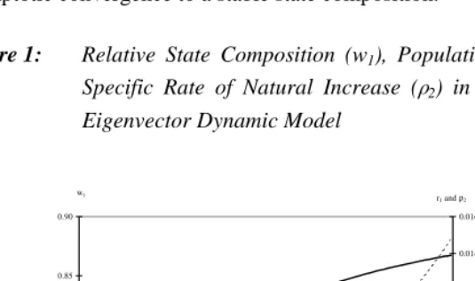
.8944). The transition is quite lengthy, however, and is still not complete after 1000 years (see Figure 1). The length of the transition is not related to the conventional speed of convergence to stability, but rather to the (arbitrary) rate of change in the transition rates (here e-.002t). The model thus describes dynamic relationships not previously known, and affords a heretofore unavailable analytical platform for examining asymptotic convergence to a stable state composition.

Figure 1: Relative State Composition (w1), Population Growth (r1), and a

State-Specific Rate of Natural Increase (S2) in a Two Living State Additive

Eigenvector Dynamic Model

0.65 0.70 0.75 0.80 0.85 0.90

0 100 200 300 400 500 600 700 800 900 1000 Time 0.000 0.002 0.004 0.006 0.008 0.010 0.012 0.014 0.016 Series2 Series1 Series3

Series4Rate of population growth in state 1 (r1) State 2 rate of natural increase (ρ2)

Size of state 2 relative to state 1 (w1)

w1 _r

1 and ρ2

w1

ρ2

5.3 Two Basic Hierarchical Proportional Eigenvector Models

Equations (14) simplify when c(t)=0. Then a*(t)=a(t), b*(t)=b(t), c*(t)=0, and d*(t) = d(t) + D ln[ {a(t)-d(t)}/b(t) ] (25) The result is a hierarchical model, in that persons can move from state 2 to state 1, but not from state 1 to state 2. Because c*(t)=c(t), it is a Proportional Eigenvector model as well.

Hierarchical models arise naturally in demography. They include models whose living states are parity status, never married and ever married, health and permanent disability, and all other instances of irreversible transitions (including multi-age models).

5.3.1 A Simple Model With Cyclical Interstate Transfer

To illustrate a basic dynamic hierarchical population, let a(t) = a*(t) = a, d(t) = d, and b(t) = b exp[f VLQ W@ZLWKFRQVWDQWVEI !7KHQ

d*(t) = d - b’(t)/b(t) = d - I FRV W and we have

[

]

a

b exp f sin t

(t)

0

d

ω





= 







(26)

and

[

]

a

b exp f sin t

(t)

0

d f cos t

ω

ω

ω





= 

₋







(27)

[

1

]

1

(t)

(d a) exp

f sin t / b

ω

0





= 

₋

₋







W

(28)

The eigenvalue matrix R(t) is a diagonal matrix whose (1,1) element is d and whose (2,2) element is a. Using equation (7), the long term state product matrix, M0,t, can be

written

[

] [

]

dt 0,t

1

e

0 b /(d a)

(d a) exp

f sin t / b

ω





=

_

_

−

−

−





M

(29)

Let x0 = w0, where w0 is the (n x 1) column vector whose elements are those of the first

column of W0. That is, let x0 be the column vector whose first element is 1 and whose

second element is (d-a)/b. Then the long term size and structure of the model are given by

[

]

d t t

1

e

d

a

b e x p f s in

ω

t













=

_

_

−













x

(30)

Because the rates of natural increase in both states are constant while b(t) varies sinusoidally, population size oscillates around an exponentially increasing trajectory,

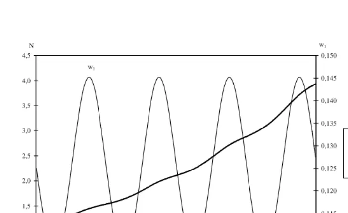
ZKLOHWKHVWDWHFRPSRVLWLRQRIWKHPRGHOF\FOHVZLWKSHULRG7 VHH)LJXUHQH[W SDJH ZKHUH D E G DQG I :H WKXV KDYH D FRPSOHWHO\

Figure 2: Relative State Composition (w1) and Total Population Size (N) for a

Hierarchical Two Living State Proportional Eigenvector Model

5.3.2 A Simple Model With Cyclical Natural Increase

Let us consider the same type of model, but with interstate transfer rate b constant and with a cyclical rate of natural increase in state 2 so that d(t) = dVLQ W+HUH

a

b

(t)

0

d sin t

ω





= 







(31)

and 0,0 0,5 1,0 1,5 2,0 2,5 3,0 3,5 4,0 4,5

0 50 100 150 200 250

Time N

0,100 0,105 0,110 0,115 0,120 0,125 0,130 0,135 0,140 0,145 0,150 w1

Total population size (N)

Size of state 2 relative to state 1 (w1)

w1

N

a

b

(t)

d cos t

0

d sin t

d sin t

a

ω

ω

ω

ω

ω













=





+



₋







(32)

)RUDUHDOLVWLFWZRVWDWHPRGHODQGZLWKFRQVWDQWV G!DQGDZHPXVWKDYHG!D

Taking x0 = w0, the long term size and structure of the model are given by

d (1 cos t ) / t

1 e

(d sin t a ) / b

ω ω

ω

−  

= _{ }

−

 

x (33)

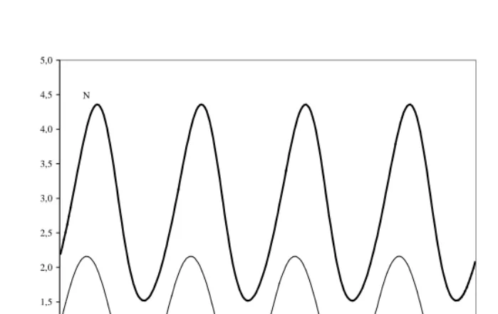
Thus when one rate of natural increase is cyclical, both the rate of growth and the state composition vary sinusoidally over time. Figure 3 illustrates the size and composition of the population when a=- E G DQG %RWK F\FOH ZLWK WKH VDPH periodicity, but they differ a bit in phase and a good deal in amplitude.

Figure 3: Relative State Composition (w1) and Total Population Size (N) for a

Cyclical Hierarchical Two Living State Model

6. Summary and Conclusion

Dynamic multistate population models recognize more than one living state and allow demographic rates to vary over time. Because the dynamic multistate model is extremely flexible, it can reflect the behavior of any observed population at any time. The state composition of a dynamic multistate population—or of an observed population—is usually seen as the consequence of a series of past rates. Nonetheless, analysis of basic differential equation (1) shows that the state composition can always be expressed in terms of current rates and current compositional change alone, without having to consider earlier time points.

By introducing the concept of latent rates, any population can be seen as only an instant away from achieving the stability implied by those rates. Finding latent rates from observed rates implies a solution to differential equation (1), which is not always

0,0 0,5 1,0 1,5 2,0 2,5 3,0 3,5 4,0 4,5 5,0

0 50 100 150 200 250

Time

Total population size (N)

Size of state 2 relative to state 1

Total population size (N)

Size of state 2 relative to state 1 (w1)

N

possible, but one can find the observed rates when the latent rates are known in functional form.

A solution to differential equation (1) is possible in two special cases. Those circumstances, one of which was not previously recognized, are discussed in some detail. Examples utilizing those solutions suggest that they offer a promising basis for empirical and analytical investigations.

In short, closed form dynamic multistate models are both possible and analytically tractable. Dynamic models are the next logical step beyond fixed rate stable models, and multi-age models can be seen as just a special case of multistate models. Rather than the unchanging stationary population of the life table, cyclical populations can emerge as a natural context for long term demographic analysis. Formal demography needs to move beyond the fixed rate assumption to capture changing relationships in a dynamic world.

Changes

On 07 January 2002, per request of the author, these three changes were made.

1) on page 171 this sentence was deleted following equation (17): Although not pointed out in Schoen and Kim (2000), the Proportional Eigenvector solution can be generalized. It applies not only when matrix C is a constant, but when C is any known, differentiable function of time.

2) on the same page the word “second” was deleted from the paragraph: A (second) previously unappreciated feature of the Proportional Eigenvector form is that it reduces to the “fixed f” dynamic multi-age approach….

References

Boyce, W.E. and R.C. DiPrima. 1977. Elementary Differential Equations and Boundary

Value Problems (3d Ed.) New York: Wiley.

Caswell, H. 1989. Matrix Population Models. Sunderland MA: Sinauer.

Gantmacher, F.R. 1959. The Theory of Matrices. Volume II. New York: Chelsea (Translated from the Russian by K.A. Hirsch).

Keyfitz, N. 1971. On the momentum of population growth. Demography 8:71-80. Keyfitz, N. 1977. Introduction to the Mathematics of Population. (2d Ed.) Reading

MA: Addison-Wesley.

Kim, Y.J and R. Schoen. 1996. Populations with quadratic exponential growth.

Mathematical Population Studies 6:19-33.

Land, K.C. and A. Rogers. 1982. Multidimensional Mathematical Demography. New York: Academic Press.

Rogers, A. 1975. Introduction to Multiregional Mathematical Demography. New York: Wiley.

Rogers, A. and F.J. Willekens. 1986. Migration and Settlement: A Multiregional

Comparative Study. Dordrecht, Holland: Reidel.

Schoen, R. 1988a. Practical uses of multistate population models. Annual Review of

Sociology 14:341-61.

Schoen, R. 1988b. Modeling Multigroup Populations. New York: Plenum.

Schoen, R and Y.J. Kim. 1994. Hyperstability. Paper presented at the Annual Meeting of the Population Association of America in Miami FL.

Schoen, R. and Y.J. Kim. 1998. Momentum under a gradual approach to zero growth.

Population Studies 52:295-99.

Schoen, R. and Y.J. Kim. 2000. A dynamic multistate model of robustness and frailty.