A hybrid method with optimal stability properties for the numerical
solution of stiff differential systems
Akram Movahedinejad
Faculty of Mathematical Sciences, University of Tabriz, Tabriz, Iran. E-mail:a [email protected]
Ali Abdi∗
Faculty of Mathematical Sciences, University of Tabriz, Tabriz, Iran. E-mail:a [email protected]
Gholamreza Hojjati
Faculty of Mathematical Sciences, University of Tabriz, Tabriz, Iran. E-mail:[email protected]
Abstract In this paper, we consider the construction of a new class of numerical methods based on the backward differentiation formulas (BDFs) that be equipped by including two off–step points. We represent these methods from general linear methods (GLMs) point of view which provides an easy process to improve their stability properties and implementation in a variable stepsize mode. These superiorities are confirmed by the numerical examples.
Keywords. Backward differentiation formula, Hybrid methods, General linear methods,A– andA(α)– stability, Variable stepsize implementation.
2010 Mathematics Subject Classification. 65L05.
1. Introduction
We shall be concerned with the construction of numerical methods for solving stiff autonomous ordinary differential equations (ODEs) of the form
y(x) =f(y(x)), y(x
0) =y0, (1.1)
on the finite intervalI:= [x0, x] where y:I→Rmandf :Rm→Rm are continuous and differentiable, andmis the dimensionality of the system. Backward differentiation formulas (BDFs) [12] are the standard and popular methods in the class of multivalue methods with the form
k
j=0
αjyn+j =hβkfn+k.
Received: 23 November 2016 ; Accepted: 3 January 2017.
∗Corresponding author.
Theses methods are A(α)–stable up to order p = k = 6 [21]. Many codes have been introduced for solving stiff initial value problems based on BDFs with good accuracy and reasonably wide region of absolute stability. Some extensions of BDFs were introduced by using the future points technique such as EBDF (extended BDF) [6], MEBDF (modified EBDF) [4], MF–MEBDF (Matrix free MEBDF) [18], A–BDF method [11] and A–EBDF method [17], by using the higher derivatives of the solutions technique such as SDBDF [5] and MESDMM [16], and also by using the off–step points such as methods introduced in [8,9,13].
In this paper, we first construct a modification of BDF which applies two off–step points technique and represent it from general linear methods (GLMs) point of view with the aim of obtaining extensive absolute stability regions. Also, we implement
A–stable methods of this category for solving stiff ODEs in a variable stepsize envi-ronment.
The rest of the paper is organized as follows: In Section2, we construct hybrid BDFs (HBDFs) including two off-step points with the aim of achieving the maximum value ofαofA(α)-stability. In section3, implementation of the methods using variable stepsize technique are investigated. Finally, in Section 4, some results of numerical experiments are presented to confirm the theoretical results.
2. Construction of HBDFs with extended stability region
In this section, we first consider a new class of numerical methods for ODEs which are based on BDFs by using two off-step points. Then, we present these methods in the form of general linear methods to obtain extensive absolute stability regions.
2.1. HBDFs with two off-step points. Assume that the solution of (1.1) has desired continuous derivatives in the interval [x0, x]. We introduce a new class of
HBDFs with two off-step points as follows
yn+k =
k
j=1
¯
αjyn+k−j+hβ¯1fn+k−θ+hβ¯2fn+k+η+hβ¯3fn+k, (2.1)
wherexn =x0+nh, n= 1,2,· · ·,his the stepsize, 0< θ <1,η >0,fn+k =f(yn+k),
fn+k−θ = f(yn+k−θ) and fn+k+η =f(yn+k+η). The coefficients ¯αj, j = 1,2, . . . , k
and ¯βj, j = 1,2,3, are computed by solving the appropriate order conditions for the orderp= k+ 1. In these methods, we need the first derivative of the solution
y(x) in two off–step points, i.e., xn+k−θ and xn+k+η. Assuming that the values of
yn, yn+1, ..., yn+k−1 are available, the method (2.1) is used in practice with applying
two predictors that take the forms
yn+k−θ= k
j=1
˜
αjyn+k−j+hβ˜1fn+k−θ, (2.2)
and
yn+k+η =
k
j=1
ˆ
where the coefficients are chosen such that equations (2.2) and (2.3) have order k. Then the approach goes as follows:
stage 1.: Use the predicator (2.2) to compute ¯yn+k−θ
¯
yn+k−θ=
k
j=1
˜
αjyn+k−j+hβ˜1f¯n+k−θ, (2.4)
where ¯fn+k−θ=f(¯yn+k−θ).
stage 2.: Use the predicator (2.3) to compute ¯yn+k+η
¯
yn+k+η = k
j=1
ˆ
αjyn+k−j+hβˆ1f¯n+k−θ+hβˆ2f¯n+k+η, (2.5)
where ¯fn+k+η =f(¯yn+k+η).
stage 3.: Computeyn+k as the solution of
yn+k = k
j=1
¯
αjyn+k−j+hβ¯1f¯n+k−θ+hβ¯2f¯n+k+η+hβ¯3fn+k. (2.6)
We note that the parameters ˆβ2, ¯β3and two parameters which determine the position
of two off step points, i.e. θandη, remain as free parameters.
Now, we are going to prove that the new method (2.4)-(2.6) has orderp=k+ 1. We assume that the local truncation errors for (2.4), (2.3) and (2.1) are
y(xn+k−θ)−y¯n+k−θ=Ck+1hk+1y(k+1)(xn) +O(hk+2), (2.7)
y(xn+k+η)−¯yn+k+η =Ck+1hk+1y(k+1)(xn) +O(hk+2), (2.8)
and
y(xn+k)−yn+k=Ck+2hk+2y(k+2)(xn) +O(hk+3), (2.9)
with the error constants Ck+1, Ck+1 and Ck+2, respectively. Thus, we have the
following theorem.
Theorem 2.1. Assume that
(1) formula (2.4)is of order k,
(2) formula (2.5)is of order k,
(3) formula (2.6)is of order k+ 1,
then, the method (2.4)–(2.6)has order k+ 1.
Proof. Suppose that the valuesyn, yn+1, . . . , yn+k−1 be exact. From (2.4) we have
Since in (2.5) we apply ¯yn+k−θ, the error of y(xn+k−θ)−y¯n+k−θ must be added to
the (2.8). Hence, using the mean value theorem and (2.10) yield
y(xn+k+η)−y¯n+k+η =hβˆ1f(y(xn+k−θ))−f(¯yn+k−θ) +Ck+1hk+1y(k+1)(xn) +O(hk+2)
=hβˆ1∂f∂y(τ)
y(xn+k−θ)−y¯n+k−θ
+Ck+1hk+1y(k+1)(xn) +O(hk+2)
=hβˆ1∂f∂y(τ)(Ck+1hk+1y(k+1)(xn))
+Ck+1hk+1y(k+1)(xn) +O(hk+2)
=Ck+1hk+1y(k+1)(xn) +O(hk+2),
whereτ is a point in the interval whose endpoints are ¯yn+k−θand y(xn+k−θ). Simi-larly, from (2.6) and by considering the errors ofy(xn+k−θ)−¯yn+k−θandy(xn+k+η)− ¯
yn+k+η to the expression of (2.9), we have
y(xn+k)−yn+k =hβ¯1
f(y(xn+k−θ))−f(¯yn+k−θ)
+hβ¯2
f(y(xn+k+η))
−f(¯yn+k+η)
+Ck+2hk+2y(k+2)(xn) +O(hk+3)
=hβ¯1∂f∂y(τ1)
y(xn+k−θ)−y¯n+k−θ+hβ¯2∂f∂y(τ2)
y(xn+k+η)
−y¯n+k+η
+Ck+2hk+2y(k+2)(xn) +O(hk+3)
=hk+2
Ck+2y(k+2)(xn) + Ck+1β¯1∂f∂y(τ1)+
Ck+1β¯2∂f∂y(τ2)
y(k+1)(x
n)
+O(hk+3).
Here,τ1andτ2are points in the interval whose endpoints areyn+k−θ andy(xn+k−θ), forτ1, andyn+k+η andy(xn+k+η), forτ2. So the order of overall method isk+ 1.
2.2. HBDFs with two off–step points as GLMs. In this subsection, at first, we express HBDFs with two off–step points from GLMs point of view. Then by using this representation, we obtain the free parameters such that the method has low implementation cost and more extensive absolute stability region.
GLMs [1,2,3,20] in each step importrquantities from the previous step and export the same number of quantities of orderpto use in the following step that denoted by
y[n−1]= [y[n−1]
i ]ri=1 andy[n]= [y[in]]ri=1, respectively. GLMs havesstages that these
values are collected in a vector denoted by Y[n] = [Y[n]
i ]si=1 and the first derivative
solution atxn−1+cihof orderq, i.e., Yi=y(xn−1+cih) +O(hq+1),
wherec= [c1, c2, . . . , cs]T is abscissae vector. The quantities imported and evaluated
in step numbernare related to
Y[n]=h(A⊗I
m)f(Y[n]) + (U⊗Im)y[n−1],
y[n]=h(B⊗I
m)f(Y[n]) + (V ⊗Im)y[n−1],
(2.11)
wheren= 1,2, ..., N, Nh=x−x0, and⊗is the Kronecker product of two matrices.
Here,A ∈ Rs×s, U ∈Rs×r, B ∈ Rr×s and V ∈Rr×r are coefficients matrices of a GLM.
Now it can be verified that the algorithm based on formulas (2.4)–(2.6) can be written as a GLM of the form (2.11) with s = 3, r =k and with the vectorsY[n], f(Y[n]) andy[n] as
Y[n]=
⎡ ⎢ ⎢ ⎣
¯
yn+k−θ
¯
yn+k+η
yn+k
⎤ ⎥ ⎥
⎦, f(Y[n]) = ⎡ ⎢ ⎢ ⎣
¯
fn+k−θ
¯
fn+k+η
fn+k
⎤ ⎥ ⎥
⎦, y[n] = ⎡ ⎢ ⎢ ⎢ ⎢ ⎢ ⎢ ⎣
yn+k yn+k−1
.. .
yn+1
⎤ ⎥ ⎥ ⎥ ⎥ ⎥ ⎥ ⎦ .
The coefficient matricesA,U,B andV are given by
A= ⎡ ⎢ ⎢ ⎣ ˜
β1 0 0
ˆ
β1 βˆ2 0
¯
β1 β¯2 β¯3
⎤ ⎥ ⎥
⎦, U= ⎡ ⎢ ⎢ ⎣
˜
α1 α˜2 · · · α˜k
ˆ
α1 αˆ2 · · · αˆk
¯
α1 α¯2 · · · α¯k
⎤ ⎥ ⎥ ⎦, B= ⎡ ⎢ ⎢ ⎢ ⎢ ⎢ ⎣ ¯
β1 β¯2 β¯3
0 0 0 .. . ... ... 0 0 0
⎤ ⎥ ⎥ ⎥ ⎥ ⎥ ⎦
, V = ⎡ ⎢ ⎢ ⎢ ⎢ ⎢ ⎢ ⎢ ⎢ ⎢ ⎣ ¯
α1 α¯2 · · · α¯k−1 α¯k
1 0 · · · 0 0
0 1 · · · 0 0
..
. ... . .. ... ...
0 0 · · · 1 0
⎤ ⎥ ⎥ ⎥ ⎥ ⎥ ⎥ ⎥ ⎥ ⎥ ⎦ ,
whereA∈R3×3,U ∈R3×k,B∈Rk×3,V ∈Rk×k andc= [1−θ,1 +η,1]T.
The coefficient matrixA plays main role in determining the implementation cost of GLMs. So, to reduce implementation cost, we assume that ˆβ2= ¯β3= ˜β1.
The stability behavior of GLMs is considered using the standard linear test problem
y =λy [7], where λis a complex parameter with negative real part. Applying test
problem to (2.11) and assuming the matrixI−zA, with z =λh, is nonsingular, we get
whereM(z) =V+zB(I−zA)−1Uis the stability matrix andp(w, z) = det(wI−M(z)) is the stability function of the method. The region of absolute stability of the method (2.11) is the subset of the complex plane
S={z∈C : all rootswi(z) ofp(w, z) are in the unit circle}.
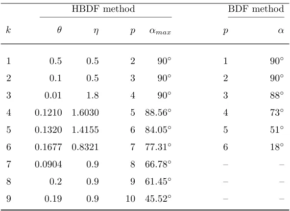
To obtain the absolute stability region of the presented methods, the boundary locus method is used. We set w = eiν, where i is the imaginary unit, with ν ∈ [0,2π] and then by usingp(w, z) = 0, we obtain three roots,zj(θ, η), j = 1,2,3, that give us the boundary of the stability region for the given θ and η. We next define an objective function which approximates the negative value of the angleαfor specific choices of parametersθ andη. Then by using fminsearch command from MATLAB, we minimize this objective function. The optimal values ofθ and η (preserving zero stability) and the corresponding maximum value forαare listed and compared with those in BDFs in Table 1. For these values ofθ andη, HBDFs are A–stable up to order 4 andA(α)–stable up to order 10.
Table 1. The values of optimalθ, η to obtain maximum value ofα.
HBDF method BDF method
k θ η p αmax p α
1 0.5 0.5 2 90◦ 1 90◦
2 0.1 0.5 3 90◦ 2 90◦
3 0.01 1.8 4 90◦ 3 88◦
4 0.1210 1.6030 5 88.56◦ 4 73◦
5 0.1320 1.4155 6 84.05◦ 5 51◦
6 0.1677 0.8321 7 77.31◦ 6 18◦
7 0.0904 0.9 8 66.78◦ – –
8 0.2 0.9 9 61.45◦ – –
9 0.19 0.9 10 45.52◦ – –
3. Implementation of the methods in a variable stepsize mode
3.1. Nordsieck representation of the HBDFs. In this subsection, we derive the Nordsieck representation of HBDFs which makes easy to implement in a variable step size environment. Nordsieck representation is achieved by forcing the vectors of incoming and outgoing to directly approximate of the Nordsieck vector
z(xn, h) := ⎡ ⎢ ⎢ ⎢ ⎢ ⎢ ⎢ ⎣
y(xn)
hy(xn)
.. .
hpy(p)(x
n) ⎤ ⎥ ⎥ ⎥ ⎥ ⎥ ⎥ ⎦ ,
of orderp. The number of incoming and outgoing approximations in the HBDFs in the GLMs form isr=k. For the vectory[n]of external vector approximates directly
the Nordsieck vector z(xn, h), we add two extra independent components hfn+k−θ andhfn+k+η to the output vector, i.e.,
y[n]=
⎡ ⎢ ⎢ ⎢ ⎢ ⎢ ⎢ ⎢ ⎢ ⎢ ⎢ ⎢ ⎢ ⎣
yn+k yn+k−1
.. .
yn+1 hfn+k−θ hfn+k+η
⎤ ⎥ ⎥ ⎥ ⎥ ⎥ ⎥ ⎥ ⎥ ⎥ ⎥ ⎥ ⎥ ⎦ .
With this change the coefficient matricesU,B, andV take the following forms
U = ⎡ ⎢ ⎢ ⎣ ˜
α1 α˜2 · · · α˜k 0 0
ˆ
α1 αˆ2 · · · αˆk 0 0
¯
α1 α¯2 · · · α¯k 0 0
⎤ ⎥ ⎥ ⎦, B= ⎡ ⎢ ⎢ ⎢ ⎢ ⎢ ⎢ ⎢ ⎢ ⎢ ⎢ ⎢ ⎣ ¯
β1 β¯2 β¯3
0 0 0 .. . ... ... 0 0 0
1 0 0
0 1 0 ⎤ ⎥ ⎥ ⎥ ⎥ ⎥ ⎥ ⎥ ⎥ ⎥ ⎥ ⎥ ⎦
, V = ⎡ ⎢ ⎢ ⎢ ⎢ ⎢ ⎢ ⎢ ⎢ ⎢ ⎢ ⎢ ⎢ ⎢ ⎢ ⎣ ¯
α1 α¯2 · · · α¯k−1 α¯k 0 0
1 0 · · · 0 0 0 0
0 1 · · · 0 0 0 0
..
. ... . .. ... ... ... ...
0 0 · · · 1 0 0 0
0 0 · · · 0 0 0 0
0 0 · · · 0 0 0 0
⎤ ⎥ ⎥ ⎥ ⎥ ⎥ ⎥ ⎥ ⎥ ⎥ ⎥ ⎥ ⎥ ⎥ ⎥ ⎦ .
For transforming the external vector to the Nordsieck vector, we define the relation
y[n]
i = p+1
j=1 tijzi[n],
wherezi[n],i= 1,2, ..., p+ 1,denote theith component of the Nordsieck vector. This transformation can be written more compactly as
y[n] =T z[n], (3.1)
where
T= ⎡ ⎢ ⎢ ⎢ ⎢ ⎢ ⎢ ⎢ ⎢ ⎢ ⎢ ⎢ ⎢ ⎢ ⎣
1 k k2!2 · · · kpp!
1 k−1 (k−2!1)2 · · · (k−p1)! p
..
. ... ... · · · ...
1 1 1
2 · · · p1!
0 1 k−θ · · · (k(−p−θ)1)!p−1
0 1 k+η · · · (k(+p−η)1)!p−1
⎤ ⎥ ⎥ ⎥ ⎥ ⎥ ⎥ ⎥ ⎥ ⎥ ⎥ ⎥ ⎥ ⎥ ⎦
. (3.2)
By substituting (3.1) into (2.11), we obtain
Y[n]=h(A⊗I
m)f(Y[n]) + (P⊗Im)z[n−1],
z[n]=h(G⊗I
m)f(Y[n]) + (Q⊗Im)z[n−1],
(3.3)
where the new coefficient matricesP,GandQare defined by
P=UT, G=T−1B, Q=T−1V T.
So, (3.3) is the desired Nordsieck representation of the method.
3.2. Variable stepsize formulation of HBDFs. For the variable step formulation of the methods on a nonuniform grid
x0< x1<· · ·< xN, xN ≥x,
the Nordsieck representation of the method takes the form
Y[n] =h
n(A⊗Im)f(Y[n]) + (PD(δn)⊗Im)z[n−1],
z[n]=h
n(G⊗Im)f(Y[n]) + (QD(δn)⊗Im)z[n−1],
(3.4)
n= 1,2, ..., N, where hn =xn−xn−1. HereY[n] is an approximation ofy(xn−1+ chn) = [y(xn−1+cihn)]si=1,y[n]is an approximation of orderpto the Nordsieck vector
[hin−1y(i−1)(xn)]pi=1+1, andD(δn) is the rescaling matrix defined by
D(δn) := diag1, δn, δn2, . . . , δnp
, δn=hn/hn−1.
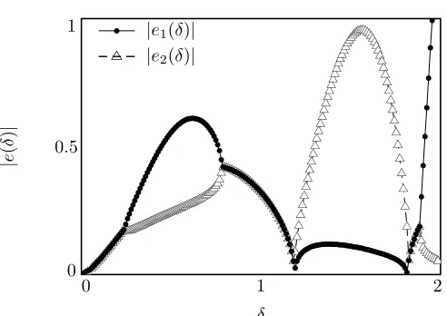
method with k= 1, the eigenvalues of matrix QD(δ) are 1,0,0 and so the method is zero stable for any variable step size pattern. Fork= 2, the eigenvalues ofQD(δ) are 1,0,0 and e(δ) where e(δ) = 1.751477121δ−2.433631368δ2+ 0.8603747259δ3. For any givenδ in the interval [0,2.128764453], eigenvaluee(δ) is smaller than one. And fork= 3, the eigenvalues ofQD(δ) are 1,0,0, e1(δ) ande2(δ). We have plotted the values ofe1(δ) and e2(δ) for δ ∈ [0,2] in Figure1. For everyδ in the interval [0,1.949578008], eigenvaluese1(δ) ande2(δ) are smaller than one.
Figure 1. The plot of|e(δ)| versusδ.
δ | e ( δ ) | 0 0 1
0.5
2 1
• |e1(δ)|
|e2(δ)|
For any method to be implemented in variable stepsize mode it must be estimated the local truncation error, as this allows a measure of how accurate the approximations are, and how much the stepsize should be varied. The local truncation error is given by
Ep+1hp+1y(p+1)(xn) +O(hp+2),
whereEp+1 is the error constant for the method of orderpand determine with
p(exp(z), z) =Ep+1zp+1+O(zp+2). (3.5)
Assuminghis sufficiently small, we approximatehp+1y(p+1)(x
n) so that
LTE(xn) =Ep+1hp+1y(p+1)(xn), (3.6) can be calculated as an approximation to the local truncation error. It is possible to approximate the estimation ofhp+1y(p+1)(x
n) with a linear combination of the known stage derivatives,hf(Yi[n]),i= 1,2,3 and some components of the input vector. So an approximation to (3.6) can be represented by
est(xn) :=Ep+1 3
i=1
ηpihf(Yi[n]) + p−2
i=1
γpiy[in+3−1]
For the method withk= 1 andp= 2, we haveE3=241 and η21= 4, η22= 4, η23=−8.
For the method withk= 2 andp= 3, we haveE4=227861760002608179043 and
η31=
500
17 , η32= 100
17, η33=− 600
17, γ31=− 15 17. For the method withk= 3 andp= 4, we haveE5= 0.0564 and
η41=8000000009883867 , η42= 4000000088954803, η43=−40000000491463 ,
γ41=−4000054607, γ42=−163821191600.
Now, we recall the implementation strategies which have been investigated in [19] to apply in our numerical experiments.
The used strategy to control the stepsize in the advancing from the stepnto the stepn+ 1 is according to the following control
est(xn)≤Rtol·max{yn,yn+1}+Atol, (3.7) where Atol and Rtol are given the absolute and relative tolerances. If the control (3.7) is not satisfied, the current step is repeated with the halved stepsize. Otherwise, the current step is accepted and we use the standard step control strategy (see [14]) as the following
hn+1= min
∆,
ρ·tol
est(xn)
1 p+1
hn.
Also, in our numerical experiments, we have usedAtol=Rtol=tol,ρ= 0.95 and ∆ = 2 fork= 1,2 and ∆ = 1.8 fork= 3.
4. Numerical experiments
In this section, the constructed methods are verified by some numerical experiments in a variable stepsize environment.
We consider the following test problems:
Problem 1. Non–linear stiff ordinary differential equation [10] ⎧
⎪ ⎪ ⎨ ⎪ ⎪ ⎩
y
1=−0.04y1+ 104y2y3−0.96 exp(−x), y
2= 0.04y1−104y2y3−107y22−0.04 exp(−x), y
3= 3×10⁷y22+ exp(−x),
withy(0) = [1,0,0]T andx∈[0,105].
Problem 2. The Van der Pol’s oscillator problem described in [15] ⎧
⎨ ⎩
y
1=y2, εy
2=
1−y12y2−y1,
Using the mentioned strategies given in section3, we have implemented HBDF of orders 2, 3 and 4 in variable stepsize environment for solving Problems 1 and 2. In Tables2-7, we have reportednsas the number of steps,nrsas the number of rejected steps, nfe as the number of function evaluations, nJe as the number of Jacobian evaluations and ge as the global error at the end of the interval of integration for different given tolerances,tol.
The numerical results confirm the capability and efficiency of the proposed meth-ods.
Table 2. Numerical results for Problem 1 solved by the method of order 2 withh0= 10−5.
tol ns nrs nfe ge
10−2 36 0 512 1.59×10⁻²
10−4 50 0 740 1.21×10⁻³
10−6 133 0 1701 8.11×10⁻⁵
10−8 529 0 6367 4.19×10⁻⁶
Table 3. Numerical results for Problem 1 solved by the method of order 3 withh0= 10−5.
tol ns nrs nfe ge
10−2 54 0 1438 1.75×10⁻²
10−4 66 0 950 1.24×10⁻³
10−6 113 0 1257 5.54×10⁻⁵
10−8 299 0 3326 2.02×10⁻⁶
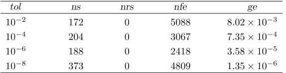
Table 4. Numerical results for Problem 1 solved by the method of order 4 withh0= 10−5.
tol ns nrs nfe ge
10−2 172 0 5088 8.02×10⁻³ 10−4 204 0 3067 7.35×10⁻⁴ 10−6 188 0 2418 3.58×10⁻⁵
Table 5. Numerical results for Problem 2 solved by the method of order 2 withh0= 10−5.
tol ns nrs nfe ge
10−2 23 1 247 9.24×10⁻²
10−4 67 0 585 5.17×10⁻³
10−6 535 2 4803 4.55×10⁻⁴
10−8 1656 3 14922 4.40×10⁻⁶
Table 6. Numerical results for Problem 2 solved by the method of order 3 withh0= 10−5.
tol ns nrs nfe ge
10−2 54 4 653 1.16×10⁻¹
10−4 94 1 1014 5.07×10⁻³
10−6 271 8 2580 2.14×10⁻⁴
10−8 1109 9 10053 8.80×10⁻⁶
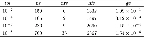
Table 7. Numerical results for Problem 2 solved by the method of order 4 withh0= 10−5.
tol ns nrs nfe ge
10−2 150 0 1332 1.09×10⁻¹
10−4 166 2 1497 3.12×10⁻³ 10−6 286 9 2690 1.15×10⁻⁴ 10−8 760 35 6367 1.54×10⁻⁶
5. Conclusion
We considered a modified version of BDFs with two off–step points in the form of GLMs. This representation made it easier to improve the stability properties of the methods such that the constructed methods are A–stable up to order 4 and A(α )-stable up to order 10 with larger angles. To apply the methods with the variable stepsize strategy, we converted the methods to the Nordsieck form. We showed that the constructed methods are practical by their implementation in variable stepsize environment on two stiff initial value problems.
References
[1] J.C. Butcher, On the convergence of numerical solutions to ordinary differential equations, Math. Comp.,20(1966), 1–10.
[4] J.R. Cash, The integration of stiff initial value problems in ODEs using modified extended backward differentiation formula, Comput. Math. Appl.,9(1983), 645–657.
[5] J.R. Cash, Second derivative extended backeward differentation formula for the numerical in-tegration of stiff systems, SIAM J. Numer. Anal.,18(1981), 21–36.
[6] J.R. Cash,On the integration of stiff systems of ODEs using extended backward differentiation formula, Numer. Math.,34(1980), 235–246.
[7] G. Dahlquist,A special stability problem for linear multistep methods, BIT,3(1963), 27–43. [8] M. Ebadi and M.Y. Gokhale, Hybrid BDF methods for the numerical solutions of ordinary
differential equations, Numer. Algor.,55(2010), 1–17.
[9] A.K. Ezzeddine and G. Hojjati,Hybrid Extended Backward Differentiation Formulas for Stiff Systems, Int. J. Nonlinear Science,12(2011), 196–204.
[10] J.E. Frank and P.J. Van Der Houwen,Parallel iteration of the extended backward differentiation formulas, IMA Journal of Numerical Analysis,21(2001), 367–385.
[11] C. Fredebeul, A–BDF: A generalization of the backward differentiation formulae, SIAM J. Numer. Anal.,12(1998), 1917–1938.
[12] W.C. Gear,Simultaneous Numerical Solution of Differential Algebraic Equation, IEEE Trans-action on Circuit Theory,18(1971), 89–95.
[13] W.C. Gear,Hybrid methods for initial value problems in ordinary differential equations, SIAM J. Numer. Anal.,2(1965), 69–86.
[14] E.Hairer, S.P. Nørsett and G. Wanner, Solving Ordinary Differential Equations I: Nonstiff Problems, Springer, Berlin, 2000.
[15] E. Hairer and G. Wanner,Solving Ordinary Differential Equations II. Stiff and Differential– Algebraic Problems, Second Revised Edition. Springer Verlag, Berlin, Heidelberg, New York, 1996.
[16] G. Hojjati, M. Rahimi and S.M. Hosseini,New second derivative multistep methods for stiff systems, Appl. Math. Model.,30(2006), 466–476.
[17] G. Hojjati, M. Rahimi and S.M. Hosseini,A–EBDF: an adaptive method for numerical solution of stiff systems of ODEs, Math. Comput. Simul.,66(2004), 33–41.
[18] G. Hojjati and S. M. Hosseini,Matrix–free MEBDF method for numerical solution of systems of ODEs, Math. Comput. Model.,29(1999), 67–77.
[19] S.J.Y. Huang,Implementation of general linear methods for stiff ordinary differential equations, PhD thesis, Department of Mathematics, Auckland University, 2005.
[20] Z. Jackiewicz,General linear methods for ordinary differential equations, Wiley, New Jersey, 2009.