A new method based on fourth kind Chebyshev wavelets to a fractional-order model of HIV infection of CD4+T cells

(1)

A new method based on fourth kind Chebyshev wavelets to a fractional–

order model of HIV infection of CD4

+

T cells

Haman Deilami Azodi∗ Faculty of Mathematical Sciences, University of Guilan, Rasht, Iran. E-mail: [email protected]

Mohammad Reza Yaghouti Faculty of Mathematical Sciences, University of Guilan, Rasht, Iran. E-mail: [email protected]

Abstract This paper deals with the application of fourth kind Chebyshev wavelets (FKCW) in solving numerically a model of HIV infection of CD4+_{T cells involving Caputo}

fractional derivative. The present problem is a system of nonlinear fractional diﬀerential equations. The goal is to approximate the solution in the form of FKCW truncated series. To do this, an operational matrix of fractional integration is constructed for these wavelets. This matrix transforms the problem to a nonlinear system of algebraic equations. Solving the new system, enables one to identify the unknown coeﬃcients of expansion. Numerical results are compared with other existing methods to illustrate the applicability of the method.

Keywords. Fourth kind Chebyshev wavelets, HIV model, Caputo derivative.

2010 Mathematics Subject Classification. 65T60, 34A08.

1. _Introduction

The human immunodeficiency virus (HIV) is a virus that attacks the immune system which is our body’s natural defense against the diseases. This virus destroys a type of white blood cells in the immune system called CD4+T and makes copies of itself inside these cells. AIDS is a status which the immune system is too weak to fight off infection.

The dynamics of CD4+_{T cells and HIV interaction are formulated by the following}

system of ordinary diﬀerential equations [27] 

     

dT

dt =p−αT+rT (

1−_TT+I

max

)

−kV T,

dI

dt =kV T −βI, dV

dt =N βI−γV,

(1.1)

Received: 11 July 2017 ; Accepted: 9 May 2018.

∗Corresponding author.

(2)

with the initial conditions

T(0) =T0, I(0) =I0, V(0) =V0. (1.2)

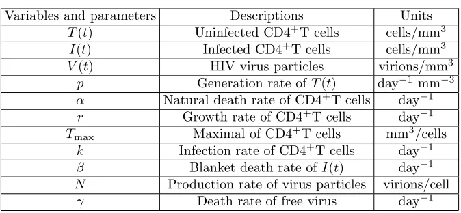
The descriptions of variables and parameters of (1.1) are listed in Table1.

Table 1. Variables and Parameters

Variables and parameters Descriptions Units

T(t) Uninfected CD4+T cells cells/mm3

I(t) Infected CD4+_{T cells} _cells/mm3 V(t) HIV virus particles virions/mm3

p Generation rate ofT(t) day−1 _mm−3 α Natural death rate of CD4+T cells day−1

r Growth rate of CD4+_{T cells} _day−1 Tmax Maximal of CD4+T cells mm3/cells

k Infection rate of CD4+_{T cells} _day−1 β Blanket death rate ofI(t) day−1

N Production rate of virus particles virions/cell

γ Death rate of free virus day−1

The mathematical model (1.1) represents the changes of infected CD4+_{T cells,}

uninfected CD4+_{T cells and virus particles numbers in a period of time. In medical}

sciences, the computation of these variables are vital to measure the progression of disease and to get a better cure. Accordingly, the numerical solution of the HIV model is a considerable task of mathematicians. The methods existing in the literature to solve (1.1) with the initial conditions (1.2) include as follows: Laplace Adomian decomposition method [20], Multi –step Laplace Adomian decomposition method [5], Variational iteration method [16], Diﬀerential transform method [25], Homotopy perturbation method [17], Bessel collocation method [31], Legendre wavelets method [26] and Taylor’s series method [11].

The important point to note here is that biological systems have memory and aftereffects. In the models interpreted by ordinary differential equations with integer-order, such effects are neglected. Because of the relation of fractional calculus to the systems with memory, fractional models are more suitable for biological systems. Thus, by replacing the integer-order derivative in (1.1) with Caputo fractional derivative, the following model is established

    

Dν1

∗ T =p−αT +rT (

1− T+I Tmax

)

−kV T, Dν2

∗ I=kV T −βI,

Dν3

∗ V =N βI−γV,

(1.3)

with the same initial conditions (1.2), where 0< ν1, ν2, ν3≤1 andD∗ denotes the

Caputo fractional derivative. For ν1 = ν2 = ν3 = 1, (1.3) reduces to the classical

(3)

See [4,21].

For solving the fractional model (1.3), Gökdogan et al. have presented a multi– step differential transform method [7], Haq et al. have used Adomian decomposition method [8] and also Gandomani et al. have proposed Müntz–Legendre polynomials collocation method [6].

From recent decades up to now, wavelet methods have been accounted as powerfool tools with diverse applications in science and technology. Especially, wavelets generated by the dilation and translation of orthogonal polynomials have been considered more than other ones in finding the solution of various types of differential and integral equations. The useful characteristics of wavelets can be summarized as follows: (a) Wavelet methods are appropriate for the computer programming. (b) The operational matrix achieved by wavelets exhibits sparsity which is computationally very fast. (c) By applying wavelets, it is possible to obtain a good approximation of a function by using only a few coefficients. (d) For a large number of the basis functions, most of the wavelet coefficients vanish. (e) The solution is multi–resolution [2,3].

As we know, there are four kinds of Chebyshev polynomials. All of them are used widely in approximation theory. They are orthogonal on [−1,1] with respect to different weight functions [15]. The operational matrices of the fractional integration related to first and second kind Chebyshev wavelets have been constructed to the numerical solution of fractional differential equations in [13] and [28], respectively. Recently, Zhou et al. have been gained an operational matrix of fractional integration of third kind Chebyshev wavelets for solving fractional convection–diffusion equation [32]. FKCW have been paid less attention by authors and no serious attempt has been made to extend FKCW for solving fractional problems. Motivated by the mentioned works, our main aim is to develope the applications of FKCW in approximation of the solution of (1.3). For this purpose, using collocation method, an operational matrix of fractional integration for FKCW is first fabricated. This matrix converts (1.3) to a nonlinear system of algebraic equations. After solving the new system by any standard iterative scheme, the solution of problem is acquired in terms of FKCW. Numerical results of the method are compared with some recent methods. Since the exact solution of (1.3) is unknown, residual errors of (1.3) are evaluated to indicate the efficiency of method.

The remainder of this paper proceeds as follows: In section2, FKCW and some properties of them are described. Uniform convergence and error estimation of FKCW expansion are also investigated. Section 3 implements the numerical method for solving (1.3). In section 4, numerical and graphical results of applying the present method are announced. Finally, concluding remarks are drawn in section5.

2. Some properties of FKCW

2.1. Wavelets and FKCW. Wavelets are a class of functions used to localize a given

(4)

parameterb of a mother waveletψdeﬁne the following continuous wavelets

ψa,b(x) =√1

aψ

(

x−b a

)

, a∈R+, b∈R. (2.1)

Now, supposea0>1 andb0>0 are ﬁxed and takea=a−0k andb=na−

k

0 b0 such

that k, n ∈ N. Instead of using the family of wavelets (2.1), we use the family of wavelets indexed byN, named the discrete wavelets,

ψk,n(x) =a k

2

0ψ

(

ak0x−nb0

)

, k, n∈N. (2.2)

The family of (2.2) constitutes an orthogonal basis onL2₍_R_{) and by choosing}_a 0= 2

andb0= 1,this basis will be an orthonormal basis on L2(R) [14,18].

FKCW are deﬁned on [0,1] forn= 1, ...,2k−1_, _k_∈_N_,_m_{= 0}_{, ..., M} ₋_1,_M _∈_N_as

ψn,m(t) = { √

1

π2

k

2W_m(2kt−2n+ 1), n−1

2k−1 ≤t <

n

2k−1,

0, otherwise, (2.3)

in whichWm are Chebyshev polynomials of fourth kind of degreem= 0,1, . . . that

are orthogonal with respect to the weight function ω(t) = √

1−t

1+t on [−1,1] and for

m∈Ncan be determined by the following recurrence formula [15]

W0(t) = 1, W1(t) = 2t+ 1, Wm+1(t) = 2tWm(t)−Wm−1(t).

The coeﬃcient √

1

π in (2.3) is for normality. The dilation and translation parameters are a = 2−k _and _b _{= (2}_n₋₁₎₂−k_, _{respectively. Also,} _k _∈ _N _{denotes the level of} resolution.

It is worth mentioning that FKCW deﬁned in (2.3) constitute an orthonormal basis onL2_[0_,_{1] with respect to the weight function}_ω

n(t) =ω (

2k_t₋₂_n_{+ 1})_.

2.2. Function approximation. Any function f(t) ∈ L2

ω[0,1] can be expanded at the levelk∈Nas

f(t) =

2k−1

∑

n=1

∞ ∑

m=0

fn,mψn,m(t), (2.4)

where

fn,m=⟨f(t), ψn,m(t)⟩_L2

ω[0,1] =

∫ 1

0

f(t)ψn,m(t)ωn(t)dt,

in which⟨., .⟩_L2

ω[0,1] denotes the inner product inL 2

ω[0,1].

Usually, the inﬁnite series in (2.4) is truncated and written in the following

f(t)≈

2k−1

∑

n=1

M_∑−1

m=0

(5)

which approximates f(t) as a ﬁnite linear combination of FKCW. In (2.5), F and

Ψ(t) are column vectors with ˆm= 2k−1M entries given by

F=[f1,0, . . . , f1,M₋1, . . . , f2k−1_,₀, . . . , f₂k−1_,M₋₁

]T

,

Ψ(t) =[ψ1,0(t), . . . , ψ1,M₋1(t), . . . , ψ2k−1_,₀(t), . . . , ψ₂k−1_,M₋₁(t)

]T

.

The following proposition ensures the uniform convergence of FKCW expansion.

Proposition 2.1. Assume f(t) be a continuous function and R = sup|f′′(t)| on

[0,1].Then, it can be expanded as an infinite sum of FKCW and the series converges uniformly tof(t), that is

f(t) =

2k−1

∑

n=1

∞ ∑

m=0

fn,mψn,m(t).

Moreover, form >1,

|fn,m|< 1 2 √ π 2 R

n52(m−1)2

.

Proof. The coeﬃcients of FKCW expansion off(t) are deﬁned as

fn,m=⟨f(t), ψn,m(t)⟩_L2

ω[0,1]

= ∫ 1

0

f(t)ψn,m(t)ωn(t)dt

= √ 1 π2 k 2 ∫ n

2k−1

n−1 2k−1

f(t)Wm (

2kt−2n+ 1)ω(2kt−2n+ 1)dt.

Letx= 2k_t₋₂_n_{+ 1. Thus,}

fn,m= √ 1 π2 −k 2 ∫ 1 −1 f (

x+ 2n−1 2k

)

Wm(x)ω(x)dx.

Puttingx= cosθentails

fn,m= √ 1 π2 −k 2 ∫ π 0 f (

cosθ+ 2n−1 2k

)

sin(m+1₂)θ

sin1₂θ

√

1−cosθ

1 + cosθsinθdθ.

Knowing √

1−cosθ

1+cosθsinθ= 2 sin

2θ

2 yields

fn,m= 2 √ 1 π2 −k 2 ∫ π 0 f (

cosθ+ 2n−1 2k

) sin

(

m+1 2

)

θsin1 2θdθ = √ 1 π2 −k 2 ∫ π 0 f (

cosθ+ 2n−1 2k

)

(cosmθ−cos(m+ 1)θ)dθ.

With the aid of integration by parts technique, it follows

fn,m= √

1

π2

−3k

2 1 m ∫ π 0 f′ (

cosθ+ 2n−1 2k

)

sinmθsinθdθ

−

√ 1

π2

−3k

2 1

m+ 1 ∫ π

0 f′

(

cosθ+ 2n−1 2k

)

sin(m+ 1)θsinθdθ.

(6)

Letζ1=_m1

∫π

0 f′

(_cos_θ₊₂_n₋₁

2k

)

sinmθsinθdθ.Then,

ζ1=

1 2m ∫ π 0 f′ (

cosθ+ 2n−1 2k

)

(cos(m−1)θ−cos(m+ 1)θ)dθ

= 2 −k 2m ∫ π 0 f′′ (

cosθ+ 2n−1 2k

) (

sin(m−1)θ m−1 −

sin(m+ 1)θ m+ 1

) sinθdθ.

Obviously,

|ζ1| ≤

1 2m2

−k_R ∫ π

0

sin(m−1)θ m−1 −

sin(m+ 1)θ m+ 1

|sinθ|dθ

≤ 1

2m2

−k₍_πR₎ (

1

m−1+ 1

m+ 1 )

< 2

−k_Rπ

(m−1)2.

Letζ2=_m1₊₁

∫π

0 f′

(_cos_θ₊₂_n₋₁

2k

)

sin(m+ 1)θsinθdθ.In a similar way,

|ζ2| ≤

2−k_Rπ

m(m+ 1) <

2−k_Rπ (m−1)2.

Now, form >1,

|fn,m| ≤ √

1

π2

−3k

2 (|ζ₁|+|ζ₂|)<

√ 1

π2

−3k

2 2×2

−k_Rπ

(m−1)2 =

2R√π

(m−1)22

−5k

2 .

Sincen≤2k−1_{, it is clear that 2}−5k

2 ≤(2n)−

5

2_{. Hence,}

|fn,m|< 1 2 √ π 2 R

n52(m−1)2

.

Ifm= 1, according to (2.6),

|fn,1| ≤

√ 1

π2

−3k

2

(

π+π 2 )

sup|f′(t)| ≤ 3 4

√

π

2

sup|f′(t)|

n32

.

So,∑2_nk−₌₁1∑∞_m₌₀fn,mis absolutely convergent and the inﬁnite sum of FKCW converges

tof(t) uniformly.

The proposition below seeks an upper bound for the error estimation of FKCW expansion.

Proposition 2.2. Under the assumptions of Proposition (2.1), assume the truncated

seriesfk,M(t) = ∑2_nk−₌₁1∑M_m₌₀−1fn,mψn,m be the FKCW approach of f(t)at the level

kfor a given M. Then,

∥f(t)−fk,M(t)∥<  π

8R

2 2∑k−1

n=1

∞ ∑

m=M 1

n5₍_m₋₁₎4

 

1 2

(7)

Proof. Using the orthonormality ofψn,m and Proposition2.1, the following relations are held.

∥f(t)−fk,M(t)∥

2

= ∫ 1

0

2

k−1

∑

n=1

∞ ∑

m=M

fn,mψn,m(t)

2ωn(t)dt

=

2k−1

∑

n=1

∞ ∑

m=M

|fn,m|

2

< π

8R

2 2k−1

∑

n=1

∞ ∑

m=M 1

n5₍_m−₁₎4.

Intuitively, iff(t) = 1

π2sin(πt) thenR= 1 and Proposition2.2reveals

∥f(t)−f1,3(t)∥<0.1798, ∥f(t)−f1,7(t)∥<0.0278, ∥f(t)−f1,13(t)∥<0.0093.

Thus, we deduce at the levelk for large enough value ofM, fk,M→f(t). For a ﬁxedM,we aﬃrm

f(t) = ∞ ∑

n=1

M∑−1

m=0

fn,mψn,m(t).

Likely, one can prove for a givenM by increasingkthe accuracy of the approximation ∑2k−1

n=1

∑M₋1

m=0fn,mψn,m(t) is improvable.

2.3. Operational matrix of fractional integration (OMFI). OMFI of a family

of wavelets can be obtained with or without Block-Pulse functions (BPF). For obtaining OMFI of Bernoulli wavelets, Keshavarz et al. expanded these wavelets into Bernoulli polynomials [10]. Then, the authors specified a relation for OMFI of Bernoulli wavelets fork = 2 and arbitraryM. Moreover, Rong et al. formed Jacobi wavelets based on the explicit formula of Jacobi polynomials [24]. Then, they found an OMFI for Jacobi wavelets. In both of these works, the designed operational matrices contain many entries in the form of summation. Thus, although OMFI works efficiently but for not so small values ofkandM, it has large computational effort.

In [1,13,19,22,23,28–30,32], OMFI has been constructed for Haar, ﬁrst kind Chebyshev, Shannon, Legendre, Gegenbauer, second kind Chebyshev, Euler, CAS and third kind Chebyshev wavelets, respectively by using BPF. The main idea in all of these references is that the corresponding wavelets family is ﬁrst expanded into BPF. Then, OMFI of BPF is used for calculating the OMFI of the wavelet. The resulting OMFI has a simple formula and is easy to perform for every k and M.

Motivated by the works mentioned above, we intend to determine OMFI of FKCW using BPF.

(8)

2.3.1. BPF.

Definition 2.3. The ˆm-set of BPF on [0,1] is deﬁned in the following

bi(t) = {

1, i−_m_ˆ1 ≤t < _m_ˆi,

0, otherwise,

wherei= 1, . . . ,m.ˆ

Remark 2.4. BPF are disjoint and orthogonal, namely

• bi(t)bj(t) = {

0, i̸=j,

bi(t), i=j,

• ∫1

0 bi(t)bj(t)dt=

{

0, i̸=j, 1

ˆ

m, i=j.

The functionf(t)∈L2[0,1] can be written as

f(t)≈

ˆ

m ∑

i=1

fibi(t) =fTBm(ˆ t),

wheref = [f1, f2, . . . , fmˆ]

T

, Bmˆ(t) = [b1(t), b2(t), . . . , bmˆ(t)]

T

,fori= 1, . . . ,mˆ

fi = ˆm ∫ 1

0

f(t)bi(t)dt.

Definition 2.5. The tensor product of two vectorsfmˆ = [fi] andgmˆ = [gi] is deﬁned

as

f⊗g= (fi×gi)mˆ .

Similarly, for two matricesA= [ai,j] andB= [bi,j] of ˆm×mˆ

A⊗B= (ai,j×bi,j)mˆ_×mˆ .

The Lemma below will be needed in the next section.

Lemma 2.6. Let the functions f(t), g(t)∈ L2[0,1] be expanded into BPF, that is

f(t) =fTBm(ˆ t)andg(t) =gTBm(ˆ t). Then

f(t)g(t) =(fT ⊗gT)Bm(ˆ t).

Proof.

f(t)g(t) =fTBm(ˆ t)BTmˆ(t)g=f1g1b1(t) +f2g2b2(t) +. . .+fmˆgmˆbm(ˆ t)

=(fT ⊗gT)Bmˆ(t).

For the sake of simplicity, we rewrite (2.5) as

f(t)≈

ˆ

m ∑

i=1

(9)

where fi =fn,m, ψi =ψn,m. The indexi is determined by i = (n−1)M +m+ 1, and ˆm= 2k−1_M._{By this notation, we get}

Fmˆ =

[

f1, . . . , fM|, fM+1, . . . , f2M|, . . . ,|f(2k−1₋₁₎_M₊₁, . . . , fmˆ

]T

,

Ψmˆ(t) =

[

ψ1, . . . , ψM|, ψM+1, . . . , ψ2M|, . . . ,|ψ(2k−1₋₁₎_M₊₁, . . . , ψmˆ

]T

.

Taking the collocation points ti = 2_{2 ˆ}i−_m1, i= 1, . . . ,mˆ, we deﬁne the ˆm×mˆ FKCW matrixΦmˆ×mˆ as

Φmˆ_×mˆ = [Ψm(ˆ t1),Ψm(ˆ t2), . . . ,Ψm(ˆ tm)]ˆ . (2.7)

2.3.2. Operational matrix. From [12], OMFI of order ν of the BPF vectorBm(ˆ t) is

oﬀered as

IνBm(ˆ t)≈Fmνˆ×mˆBm(ˆ t), (2.8)

where

Fν

ˆ

m×mˆ =

1 ˆ

mν 1 Γ(ν+ 2)

      

1 ξ1 ξ2 . . . ξmˆ−1

0 1 ξ1 . . . ξmˆ−2

0 0 1 . . . ξmˆ−3

..

. ... ... . .. ... 0 0 0 . . . 1

      

,

in whichξi= (i+ 1)ν+1−2iν+1+ (i−1)ν+1,i= 1, . . . ,mˆ −1. LetPν_m_ˆ_×_m_ˆ be the OMFI of FKCW, that is

IνΨm(ˆ t)≈Pmνˆ×mˆΨm(ˆ t), (2.9)

Now, fort∈{2_{2 ˆ}i−_m1|i= 1, . . . ,mˆ}, using (2.7) implies that

Ψm(ˆ t) =Φmˆ×mˆBm(ˆ t). (2.10)

By (2.8) and (2.10), one can write

IνΨmˆ(t) =IνΦmˆ×mˆBmˆ(t) =Φmˆ×mˆIνBmˆ(t)≈Φmˆ×mˆFmνˆ×mˆBmˆ(t). (2.11)

Also, with the aid of (2.10), we get

Bmˆ(t) =Φ−mˆ1×mˆΨmˆ(t). (2.12)

Consequently, from (2.11) and (2.12), it follows

IνΨm(ˆ t)≈Φmˆ_×mˆFνmˆ×mˆΦ− 1 ˆ

m×mˆΨm(ˆ t). (2.13)

Comparison (2.13) with (2.9) results in

Pνmˆ_×mˆ ≈Φmˆ×mˆFνmˆ_×mˆΦ− 1 ˆ

(10)

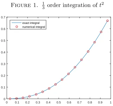
Figure 1. 13 order integration oft 2

t

0 0.1 0.2 0.3 0.4 0.5 0.6 0.7 0.8 0.9 1 0

0.1 0.2 0.3 0.4 0.5 0.6 0.7

exact integral numerical integral

which is independent ofBm(ˆ t).

Particularly, fork= 2, M = 3, ν= 0.7,OMFI of FKCW is computed as

P0₆._×7₆=        

0.2329 0.1683 −0.0142 0.5558 −0.0602 0.0116 0.0416 0.1574 0.0913 0.6457 −0.0943 0.0211

−0.0460 −0.1031 0.1638 0.2089 −0.0537 0.0145

0 0 0 0.2329 0.1683 −0.0142 0 0 0 0.0416 0.1574 0.0913 0 0 0 −0.0460 −0.1031 0.1638

       

.

One should mention that CPU time of MATLAB software to calculateP0.7 ˆ

m×mˆ for the

values (k= 4, M = 5ormˆ = 40), (k= 6, M = 7ormˆ = 224), (k= 8, M = 9ormˆ = 1152) and (k= 10, M = 11ormˆ = 5632) is 0.0042s, 0.1170s, 3.2529s and 152.1935s, respectively. This means that OMFI of FKCW is computationally fast.

For example, considerf(t) =t2_._{The fractional integration of order}_ν _of_f _{is given}

by

Iνf(t) = Γ(3) Γ(ν+ 3)t

ν+2_.

The correctness of OMFI are shown in Figure1forν =1

3, k= 3, M= 4 or ˆm= 16.

3. _{Implementation of numerical method}

First, let us rewrite the fractional–order model of HIV infection (1.3) as 

 

Dν1

∗ T =p+ (r−α)T−Tmaxr T

2₋ r

TmaxT I−kV T,

Dν2

∗ I=kV T −βI,

Dν3

∗ V =N βI−γV.

(11)

Put

  

Dν1

∗ T(t)≈CTΨm(ˆ t), Dν2

∗ I(t)≈DTΨm(ˆ t), Dν3

∗ V(t)≈KTΨmˆ(t),

(3.2)

in which C = [c1, . . . , cm]ˆ

T

,D = [d1, . . . , dm]ˆ

T

, K = [k1, . . . , km]ˆ

T

. Integrating of fractional–order, we obtain

  

T(t) =Iν1_Dν1

∗ T(t) +T0≈CTPνmˆ1_×mˆΨm(ˆ t) +T0, I(t) =Iν2_Dν2

∗ I(t) +I0≈DTPν_m_ˆ2_×_m_ˆΨm(ˆ t) +I0, V(t) =Iν3_Dν3

∗ V(t) +V0≈KTPνmˆ3×mˆΨmˆ(t) +V0,

(3.3)

whereI(.)is the Riemann–Liouville fractional integral operator. Collocating (3.3) at the pointst∈{2_{2 ˆ}i−_m1|i= 1, . . . ,mˆ}and using (2.10) lead to

  

T(t)≈CTPν1

ˆ

m_×mˆΦmˆ×mˆBm(ˆ t) + [T0, . . . , T0]1_×mˆBm(ˆ t), I(t)≈DT_Pν2

ˆ

m×mˆΦmˆ×mˆBm(ˆ t) + [I0, . . . , I0]1×mˆBm(ˆ t), V(t)≈KT_Pν3

ˆ

m×mˆΦmˆ×mˆBmˆ(t) + [V0, . . . , V0]1×mˆBmˆ(t).

(3.4)

Let CT_Pν1

ˆ

m×mˆΦmˆ×mˆ = [a1, . . . , am]ˆ . Then, the nonlinear terms of (3.1) can be

expressed as

T2(t) =[a2₁, . . . , a2_m_ˆ]Bmˆ(t) + 2 [T0a1, . . . , T0amˆ]Bmˆ(t)

+[T₀2, . . . , T₀2]₁

×mˆBmˆ(t),

(3.5)

T(t)I(t) =([a1, . . . , am]ˆ ⊗DTPν_m_ˆ2_×_m_ˆΦmˆ_×mˆ

)

Bm(ˆ t)

+([T0, . . . , T0]1×mˆ ⊗D

T_Pν2

ˆ

m×mˆΦmˆ×mˆ

)

Bmˆ(t)

+ [T0I0, . . . , T0I0]1_×mˆ Bm(ˆ t) + [I0a1, . . . , I0am]ˆ Bm(ˆ t),

(3.6)

V(t)T(t) =([a1, . . . , amˆ]⊗KTPνmˆ3×mˆΦmˆ×mˆ

)

Bmˆ(t)

+([T0, . . . , T0]1_×mˆ ⊗K

T_Pν3

ˆ

m_×mˆΦmˆ×mˆ

)

Bm(ˆ t)

+ [T0V0, . . . , T0V0]₁_×_m_ˆBm(ˆ t) + [V0a1, . . . , V0am]ˆ Bm(ˆ t).

(3.7)

(12)

unknowns is achieved                                                     

CTΦmˆ×mˆ = [p, . . . , p]1_×mˆ + (r−α) [a1+T0, . . . , amˆ +T0]

− r

Tmax

[

a2

1+ 2T0a1+T02, . . . , am2ˆ + 2T0amˆ +T02

]

− r

Tmax

(

[a1, . . . , am]ˆ ⊗DTPνmˆ2_×mˆΦmˆ×mˆ + [I0a1, . . . , I0am]ˆ

)

− r

Tmax

(

[T0, . . . , T0]1×mˆ ⊗D

T_Pν2

ˆ

m×mˆΦmˆ×mˆ + [T0I0, . . . , T0I0]1×mˆ

)

−k([a1, . . . , am]ˆ ⊗KTPν_m_ˆ3_×_m_ˆΦmˆ_×mˆ + [V0a1, . . . , V0am]ˆ

)

−k([T0, . . . , T0]1×mˆ ⊗K

T_Pν3

ˆ

m×mˆΦmˆ×mˆ + [T0V0, . . . , T0V0]1×mˆ

)

,

DT_Φ

ˆ

m_×mˆ =k

(

[a1, . . . , am]ˆ ⊗KTPν_m_ˆ3_×_m_ˆΦmˆ_×mˆ + [V0a1, . . . , V0am]ˆ

)

+k([T0, . . . , T0]1_×mˆ ⊗K

T_Pν3

ˆ

m_×mˆΦmˆ×mˆ + [T0V0, . . . , T0V0]1_×mˆ

)

−β(DT_Pν2

ˆ

m×mˆΦmˆ×mˆ + [I0, . . . , I0]1×mˆ

)

,

KT_Φ

ˆ

m_×mˆ =

(

N βDT_Pν2

ˆ

m_×mˆ −γKTP

ν3

ˆ

m_×mˆ

)

Φmˆ_×mˆ

+ [N βI0−γV0, . . . , N βI0−γV0]1×mˆ ,

(3.8)

which is solved by Newton-Raphson method or fsolve function of MATLAB and MAPLE softwares. Substituting ci, di and ki, i = 1, . . . ,mˆ into (3.3), T(t), I(t) andV(t) are obtained.

4. _{Numerical example}

Firstly, it is notable that we perform all of the computations by MATLAB R2015a software on a 64-bit PC with 2.20 GHz processor and 8 GB memory.

Consider thatν1=ν2=ν3=ν.Also, the initial values and parameters of the system

(1.3) explained in Table1are given as follows

T0= 0.1, I0= 0, V0= 0.1, p= 0.1, α= 0.02, β= 0.3,

r= 3, γ= 2.4, k= 0.00027, Tmax= 1500, N= 10.

Letk= 3, M = 4.After solving the nonlinear system (3.8) and substituting the obtained coeﬃcients, ci, di and ki, i = 1, . . . ,mˆ into (3.3), the solution of (1.3) is speciﬁed.

Tables2,3 and4 compare the numerical results of FKCW in the caseν = 1 with those results of [17,20,31] and fourth–order Runge–Kutta (RK4) method.

Table5is devoted to the maximum diﬀerences of RK4 method from FKCW method (fork = 3, M = 4 or ˆm = 16) and Variational iteration method (16 terms) in the caseν = 1.

These amounts for Variational iteration method are as follows 

   

L_∞(TV IM) = max|TRK−TV IM|,

L_∞(IV IM) = max|IRK−IV IM|,

(13)

and for the present wavelet method are deﬁned in the following 

   

L_∞(TW M) = max|TRK−TW M|,

L_∞(IW M) = max|IRK−IW M|,

L_∞(VW M) = max|VRK−VW M|.

The results of Table5 expose that in comparison with VIM the present method is in a better agreement with RK4 method.

Figures2(A),3(A)and4(A)demonstrate the behaviour of solution for some values ofν.It is understandable that whenνtends to 1 the solution of fractional model (1.3) approaches to the solution of classical model (1.1). Figures2(B),3(B)and4(B)also conclude the present method forν = 1 is well adapted to RK4 method.

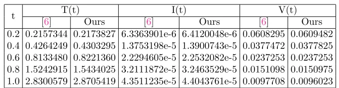
Tables 6, 7 and 8 analogy the present method to the method of [6] for ν = 0.90, 0.95, 0.98.It is visible that the results of two methods are close to each other. We can test the accuracy of FKCW method easily by using the residual errors of

T(t),I(t) and V(t) for the system (1.3). For eacht ∈[0,1], these errors are deﬁned as

    

E(T(t)) =Dν1

∗ T−p+αT −rT (

1−_TT+I

max

)

+kV T ≈0,

E(I(t)) =Dν2

∗ I−kV T+βI≈0,

E(V(t)) =Dν3

∗ V −N βI+γV ≈0.

Table9calculates absolute residual errors for ν= 0.75,k= 2 andM = 6, 9.

Figures 5, 6 and 7 portray E(T(t)), E(I(t)) and E(V(t)), respectively for k = 3, M = 4 or ( ˆm= 16) in the caseν= 0.98 by means of present method.

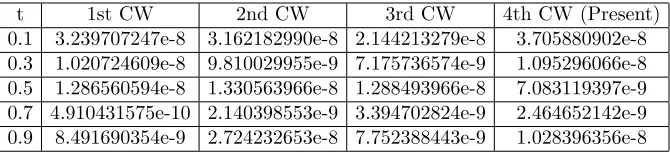
Tables 10, 11 and 12 compare absolute residual errors of 1st, 2nd and 3rd kind Chebyshev wavelets with present method for ˆm= 16 andν = 0.98.

Table 2. T(t) solutions forν= 1

t Method of [20] Method of [31] VIM [17] RK4 Present method 0.2 0.2088072731 0.2038616561 0.2088073214 0.2088080833 0.2102858565 0.4 0.4061052625 0.3803309335 0.4061346587 0.4062405393 0.4096883861 0.6 0.7611467713 0.6954623767 0.7624530350 0.7644238890 0.7720687308 0.8 1.3773198590 1.2759624442 1.3978805880 1.4140468310 1.4304307811 1.0 2.3291697610 2.3832277428 2.5067466690 2.5915948020 2.6253702046

Table 3. I(t) solutions forν = 1

(14)

Figure 2. The numerical behaviour ofT(t)

t

0 0.1 0.2 0.3 0.4 0.5 0.6 0.7 0.8 0.9 1

T(t)

0 1 2 3 4 5 6 7 8 9

ν=0.8

ν=0.85

ν=0.9

ν=0.95

ν=1

(a)Solutions ofT(t)

t

0 0.1 0.2 0.3 0.4 0.5 0.6 0.7 0.8 0.9 1

T(t)

0 0.5 1 1.5 2 2.5 3

Present method RK4 method

(b)T(t) forν= 1

Figure 3. The numerical behaviour ofI(t)

t

0 0.1 0.2 0.3 0.4 0.5 0.6 0.7 0.8 0.9 1

I(t)

×10-5

-2 0 2 4 6 8 10 12 14

ν=0.8

ν=0.85

ν=0.9

ν=0.95

ν=1

(a)Solutions ofI(t)

t

0 0.1 0.2 0.3 0.4 0.5 0.6 0.7 0.8 0.9 1

I(t)

×10-5

0 0.5 1 1.5 2 2.5 3 3.5 4 4.5

(b) I(t) forν= 1

Figure 4. The numerical behaviour ofV(t)

t

0 0.1 0.2 0.3 0.4 0.5 0.6 0.7 0.8 0.9 1

V(t)

0 0.02 0.04 0.06 0.08 0.1 0.12

ν=0.8

ν=0.85

ν=0.9

ν=0.95

ν=1

(a)Solutions ofV(t)

t

0 0.1 0.2 0.3 0.4 0.5 0.6 0.7 0.8 0.9 1

V(t)

0 0.02 0.04 0.06 0.08 0.1 0.12

(15)

Figure 5. Residual error ofT(t) for ˆm= 16, ν= 0.98

t

0 0.1 0.2 0.3 0.4 0.5 0.6 0.7 0.8 0.9 1

E(T(t))

×10-5

-1 -0.5 0 0.5 1 1.5 2 2.5 3

Figure 6. Residual error ofI(t) for ˆm= 16, ν = 0.98

t

0 0.1 0.2 0.3 0.4 0.5 0.6 0.7 0.8 0.9 1

E(I(t))

×10-5

2 2.5 3 3.5 4 4.5 5 5.5 6 6.5 7

Figure 7. Residual error ofV(t) for ˆm= 16, ν= 0.98

t

0 0.1 0.2 0.3 0.4 0.5 0.6 0.7 0.8 0.9 1

E(V(t))

×10-8

(16)

Table 4. V(t) solutions forν = 1

t Method of [20] Method of [31] VIM [17] RK4 Present method 0.2 0.0618799603 0.0618799186 0.0618799531 0.0618798433 0.0619988576 0.4 0.0383132488 0.0382949349 0.0383082013 0.0382948879 0.0383340405 0.6 0.0243917435 0.0237043186 0.0239202926 0.0237045501 0.0237076863 0.8 0.0099672189 0.0146795698 0.0162170455 0.0146803638 0.0146692185 1.0 0.0033050764 0.0237043186 0.0160841871 0.0091008450 0.0091033490

Table 5. Maximum diﬀerences of RK4 method from VIM and

present wavelet method for ν= 1

L_∞(TV IM) L∞(TW M) L∞(IV IM) L∞(IW M) L∞(VV IM) L∞(VW M) 8.48e-2 3.34e-2 1.60e-5 1.03e-7 7.00e-3 2.50e-6

Table 6. Solution forν = 0.90

t T(t) I(t) V(t)

[6] Ours [6] Ours [6] Ours

0.2 0.2501158 0.2527680 7.7692349e-6 7.8959056e-6 0.0567019 0.0568077 0.4 0.5309877 0.5377599 1.6753726e-5 1.6999140e-5 0.0358789 0.0358936 0.6 1.0784967 1.0948600 2.8164952e-5 2.8582639e-5 0.0240146 0.0240055 0.8 2.1489168 2.1869990 4.3464569e-5 4.4150437e-5 0.0168397 0.0168260 1.0 4.2409152 4.3272263 6.5030221e-5 6.6704335e-5 0.0123158 0.0124822

t T(t) I(t) V(t)

0.2 0.2272514 0.2292073 6.8290042e-6 6.9203613e-6 0.0592643 0.0593793 0.4 0.4606339 0.4653858 1.4746964e-5 1.4924381e-5 0.0369869 0.0370138 0.6 0.8979687 0.9089264 2.4155672e-5 2.4445824e-5 0.0237983 0.0237942 0.8 1.8178109 1.7431956 3.5585428e-5 3.6030591e-5 0.0157587 0.0157459 1.0 3.2590105 3.3131521 4.9905893e-5 5.0489617e-5 0.0107509 0.0106363

5. _{Concluding remarks}

(17)

t T(t) I(t) V(t)

0.2 0.2157344 0.2173827 6.3363901e-6 6.4120048e-6 0.0608295 0.0609482 0.4 0.4264249 0.4303295 1.3753198e-5 1.3900743e-5 0.0377472 0.0377825 0.6 0.8133480 0.8221360 2.2294605e-5 2.2532082e-5 0.0237253 0.0237253 0.8 1.5242915 1.5434025 3.2111872e-5 3.2463529e-5 0.0151098 0.0150975 1.0 2.8300579 2.8705419 4.3511235e-5 4.4043761e-5 0.0097708 0.0096023

Table 9. Absolute residual errors forν = 0.75 andk= 2

t |E(T(t))| |E(I(t))| |E(V(t))|

M = 6 M = 9 M = 6 M = 9 M = 6 M = 9 0.2 1.78e-7 1.89e-8 4.60e-5 4.50e-5 4.70e-8 2.95e-8 0.4 1.29e-6 1.01e-7 8.06e-5 7.85e-5 8.60e-9 1.41e-8 0.6 6.60e-5 1.82e-7 1.48e-4 1.43e-4 1.12e-7 3.23e-8 0.8 1.09e-5 4.62e-8 2.82e-4 2.71e-4 3.40e-8 1.65e-8 1.0 1.83e-3 8.28e-6 5.56e-4 5.32e-4 5.61e-7 7.33e-7

Table 10. |E(T(t))|for ˆm= 16 andν = 0.98

t 1st CW 2nd CW 3rd CW 4th CW (Present) 0.1 1.394145363e-7 2.853561788e-9 1.483582065e-7 1.173094767e-7 0.3 2.125257259e-7 3.386933558e-7 2.179188310e-7 2.162348578e-7 0.5 2.110107749e-6 2.065419183e-6 1.935604056e-6 2.334686191e-6 0.7 1.614663088e-6 1.159239888e-6 1.623875887e-6 1.405070119e-6 0.9 1.972559666e-6 1.630945443e-6 2.145168218e-6 1.920314006e-6

Table 11. |E(I(t))|for ˆm= 16 andν= 0.98

• The calculations are in the matrix form. This manner of representation makes the computer programming simple and convenient. In the other word, this method is computer–oriented.

(18)

Table 12. |E(V(t))|for ˆm= 16 andν= 0.98

• Due to the operational matrix is detected after discretization, the computation of it is done once and is used to solve fractional–order system of ordinary diﬀerential equations as well as integer–order one.

• The operational matrix simpliﬁes the problem to a solvable system of algebraic equations.

Acknowledgment

We would like to show our gratitude to the editor of journal and anonymous reviewers for their comments that greatly improved the quality of manuscript.

References

[1] Y. Chen, M. Yi., and C. Yu, Error analysis for numerical solution of fractional diﬀerential equation by Haar wavelets method, J. Comput. Sci.,3(5) (2012), 367–373.

[2] C. K. Chui,An Introduction to Wavelets, Academic Press, 1992. [3] I. Daubechies,Ten Lectures on Wavelets, SIAM, 1992.

[4] K. Diethelm,The analysis of Fractional Diﬀerential Equations, Springer–Verlag, 2010. [5] N. Dogan, Numerical treatment of the model for HIV infection of CD4+_{T cells by using}

multistep Laplace adomian decomposition method, Discrete Dyn. Nat. Soc., Article ID 976352 (2012), 11 pages.

[6] M. R. Gandomani and M. T. Kajani,Numerical solution of a fractional order model of HIV infection of CD4+_{T cells using M¨}_{untz-Legendre polynomials}_{, Int. J. Bioautomation,} ₂₀₍₂₎

(2016), 193–204.

[7] A. G¨okdogan, A. Yildirim, and M. Merdan,Solving a fractional-order model of HIV infection of CD4+_{T cells}_{, Math. Comput. Model.,}₅₄_{(9–10) (2011), 2132–2138.}

[8] F. Haq, K. Shah, G. U. Rahman, and M. Shahzad, Numerical analysis of fractional order model of HIV-1 infection of CD4+_{T-cells, Comput. Methods Diﬀer. Equ.,}₅_{(1) (2017), 1–11.}

[9] Z. Jiang and W. Schaufelberger, Block Pulse Functions and Their Applications in Control Systems, Springer-Verlag, 1992.

[10] E. Keshavarz, Y. Ordokhani, and M. Razzaghi, Bernoulli wavelet operational matrix of fractional order integration and its applications in solving the fractional order diﬀerential equations, Appl. Math. Model.,38(24) (2014), 6038–6051.

[11] M. Khalid, M. Sultana, F. Zaidi, and F. S. Khan,A Numerical Solution of a Model for HIV Infection CD4+_{T cells}_{, Int. J. Inno. Sci. Res.,}₁₆_{(1) (2015), 79–85.}

[12] A. Kilicman and Z. A. A. Al Zhour,Kronecker operational matrices for fractional calculus and some applications, Appl. Math. Comp.,187(1) (2007), 250–265.

[13] Y. Li,Solving a nonlinear fractional diﬀerential equation using Chebyshev wavelets, Commun. Nonlinear Sci. Numer. Simul.,15(9) (2010), 2284–2292.

(19)

[16] M. Merdan,Homotopy perturbation method for solving a model for hiv infection of CD4+_T cells, Istanb. Commerce Uni. J. Sci.,12(6) (2007), 39–52.

[17] M. Merdan, A. G¨okdogan, and A. Yildirim,On the numerical solution of the model for HIV infection of CD4+T cells, Comput. Math. Appl.,62(1) (2011), 118-123.

[18] M. Misiti, Y. Misiti, G. Oppenheim, and J. M. Poggi,Wavelets and their Applications, Wiley Press, 2007.

[19] K. Nouri and N. B. Siavashani, Application of Shannon wavelet for solving boundary value problems of fractional diﬀerential equations, Wavelets linear algebr.,1(1) (2014), 33–42. [20] M. Y. Ongun, The Laplace Adomian Decomposition Method for solving a model for HIV

infection of CD4+_{T cells}_{, Math. Comput. Model.,}₅₃_{(5–6) (2011), 597–603.}

[21] I. Podlubny,Fractional Diﬀerential Equations, Academic Press, 1999.

[22] M. U. Rehman and R. A. Khan,The Legendre wavelet method for solving fractional diﬀerential equations, Commun Nonlinear Sci Numer Simulat,16(11) (2011), 4163–4173.

[23] M. U. Rehman and U. Saeed, Gegenbauer wavelets operational matrix method for fractional diﬀerential equations, J. Korean Math. Soc.,52(5) (2015), 1069–1096.

[24] L. J. Rong and P. Chang,Jacobi wavelet operational matrix of fractional integration for solving fractional integro-diﬀerential equation, J. Phys. Conf. Ser, (2016), 14 pages. DOI 10.1088/1742-6596/693/1/012002.

[25] V. K. Srivastava, M. K. Awasthi, and S. Kumar,Numerical approximation for HIV infection of CD4+_{T cells mathematical model}_{, Ain Shams Eng. J.,}₅_{(2) (2014), 625–629.}

[26] S. G. Venkatesh, S. R. Balachandar, S. K. Ayyaswamy, and K. Balasubramanian, A new approach for solving a model for HIV infection of CD4+T cells arising in mathematical chemistry using wavelets, J. Math. Chem.,54(5) (2016), 1072–1082.

[27] L. Wang and M. Y. Li, Mathematical analysis of the global dynamics of a model for HIV infection of CD4+ _{T cells}_{, Math. Biosci.,}₂₀₀_{(1) (2006), 44–57.}

[28] Y. Wang and Q. Fan, The second kind Chebyshev wavelet method for solving fractional diﬀerential equations, Appl. Math. Comput.,218(17) (2012), 8592–8601.

[29] Y. Wang and L. Zhu,Solving nonlinear Volterra integro-diﬀerential equations of fractional order by using Euler wavelet method, Adv. Diﬀer. Equ., (2017), 16 pages. DOI 10.1186/s13662-017-1085-6.

[30] M. Yi and J. Huang,CAS wavelet method for solving the fractional integro-diﬀerential equation with a weakly singular kernel, Int. J. Comput. Math.,92(8) (2015), 1715–1728.

[31] S. Y¨uzbasi,A numerical approach to solve the model for HIV infection of CD4+_{T cells}_{, Appl.}

Math. Model.,36(12) (2012), 5876–5890.

[32] F. Zhou and X. Xu, The third kind Chebyshev wavelets collocation method for solving the time-fractional convection diﬀusion equations with variable coeﬃcients, Appl. Math. Comput.,